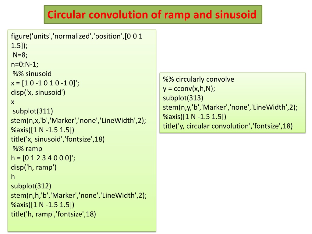
Circular Convolution of Ramp and Sinusoid

Circular convolution of a ramp signal and a sinusoid, followed by convolving a rectangular pulse with itself for exploring convolution techniques. The process involves visualizing signal convolutions, understanding how zero-padding affects plotting clarity, and using convolution for denoising a piecewise smooth signal. Additionally, convolution for edge detection is demonstrated on a piecewise smooth signal with added noise. The examples provide insights into utilizing convolution in signal processing applications.

• Signal processing
• Convolution techniques
• Denoising
• Edge detection
• Signal convolution

massman_b Follow

Uploaded on Feb 23, 2025 | 0 Views

Download Presentation

Please find below an Image/Link to download the presentation.

The content on the website is provided AS IS for your information and personal use only. It may not be sold, licensed, or shared on other websites without obtaining consent from the author.If you encounter any issues during the download, it is possible that the publisher has removed the file from their server.

You are allowed to download the files provided on this website for personal or commercial use, subject to the condition that they are used lawfully. All files are the property of their respective owners.

The content on the website is provided AS IS for your information and personal use only. It may not be sold, licensed, or shared on other websites without obtaining consent from the author.

Presentation Transcript

1. Circular convolution of ramp and sinusoid figure('units','normalized','position',[0 0 1 1.5]); N=8; n=0:N-1; %% sinusoid x = [1 0 -1 0 1 0 -1 0]'; disp('x, sinusoid') x subplot(311) stem(n,x,'b','Marker','none','LineWidth',2); %axis([1 N -1.5 1.5]) title('x, sinusoid','fontsize',18) %% ramp h = [0 1 2 3 4 0 0 0]'; disp('h, ramp') h subplot(312) stem(n,h,'b','Marker','none','LineWidth',2); %axis([1 N -1.5 1.5]) title('h, ramp','fontsize',18) %% circularly convolve y = cconv(x,h,N); subplot(313) stem(n,y,'b','Marker','none','LineWidth',2); %axis([1 N -1.5 1.5]) title('y, circular convolution','fontsize',18)

2. Convolve a rectangular pulse with itself %% pulse x = [0 0 0 1 1 1 0 0 0]'; disp('pulse') x %% convolve pulse with itself y = conv(x,x); disp('convo of pulse with itself') y % note the lengths of x and y disp('length of x'); length(x) disp('length of y'); length(y) %% zero pad x to make the pulse the same length as y for more clear plotting x(length(y)) = 0; n = 0:length(y)-1; figure('units','normalized','position',[0 0 1 1.5]); subplot(211) stem(n,x,'b','Marker','none','LineWidth',2);a xis([0 7 -1 1]); title('pulse','fontsize',18) subplot(212) stem(n,y,'b','Marker','none','LineWidth',2); title('pulse * pulse','fontsize',18)

3. Using convolution for Denoising a piecewise smooth signal close all; clear all; clc figure('units','normalized','position',[0 0 1 1.5]); %% piecewise smooth signal N = 50; n = 0:N-1; s = hamming(N) .* [ones(N/2,1); - ones(N/2,1)]; subplot(221) stem(s,'b','Marker','none','LineWidth',2); axis([1 N -1.5 1.5]) title('piecewise smooth signal','fontsize',18) %% add noise to the signal x = s + 0.1*randn(N,1); subplot(222) stem(x,'b','Marker','none','LineWidth',2); axis([1 N -1.5 1.5]) title('piecewise smooth signal + noise','fontsize',18) %% construct moving average filter impulse response of length M M=16; h = ones(M,1)/M; h1 = h; % Zero pad to let both have the same length h1(N)=0; subplot(224) stem(h1,'b','Marker','none','LineWidth',2); axis([1 N 0 1]) title('impulse response','fontsize',18) %% convolve noisy signal with impulse response y = conv(x,h); subplot(223) stem(y(M/2:N+M/2- 1),'b','Marker','none','LineWidth',2); axis([1 N -1.5 1.5]) title('output','fontsize',18)

4. Using convolution for Edge detection figure('units','normalized','position',[0 0 1 1.5]); %% piecewise smooth signal with a bit of noise added N = 50; n = 0:N-1; s = hamming(N) .* [ones(N/2,1); -ones(N/2,1)]; x = s + 0.1*randn(N,1); subplot(311) stem(x,'b','Marker','none','LineWidth',2); axis([1 N -1.5 1.5]) title('noisy piecewise smooth signal','fontsize',18) %% haar wavelet edge detector w = (1/4)*[-ones(2,1); ones(2,1)]; M = length(w); w1 = w; w1(N)=0; subplot(312) stem(w1,'b','Marker','none','LineWidth',2); axis([1 N -0.5 0.5]) title('Haar wavelet edge detector','fontsize',18) %% convolve noisy signal with impulse response y = conv(x,w); subplot(313) stem(y(M/2:N+M/2- 1),'b','Marker','none','LineWidth',2); axis([1 N -1.5 1.5]) title('output','fontsize',18)