Checking for Normality in Data Analysis
When faced with data analysis tasks involving variables whose distribution is not explicitly stated, it becomes necessary to check for normality. This involves methods like constructing histograms, assessing skewness, and detecting outliers. Through examples involving technology inventories and baseball statistics, learn how to determine if data approximates a normal distribution.

Download Presentation

Please find below an Image/Link to download the presentation.
The content on the website is provided AS IS for your information and personal use only. It may not be sold, licensed, or shared on other websites without obtaining consent from the author.If you encounter any issues during the download, it is possible that the publisher has removed the file from their server.
You are allowed to download the files provided on this website for personal or commercial use, subject to the condition that they are used lawfully. All files are the property of their respective owners.
The content on the website is provided AS IS for your information and personal use only. It may not be sold, licensed, or shared on other websites without obtaining consent from the author.
E N D
Presentation Transcript
Chapter 6: The Normal Distribution 6-4: Checking for Normality
Normally distributed variables Over the last few days, we have solved several problems involving normally distributed variables We were able to use the standard normal (z) distribution to solve these problems However, what if the problem doesn t tell you the variable is normally distributed?
Checking for Normality Histogram Pearson s Index PI of Skewness Outliers 3 Bluman, Chapter 6
Example 1: Technology Inventories A survey of 18 high-technology firms showed the number of days inventory they had on hand. Determine if the data are approximately normally distributed. 5 29 34 44 45 63 68 74 74 81 88 91 97 98 113 118 151 158 Method 1: Construct a Histogram. The histogram is approximately bell-shaped. 4 Bluman, Chapter 6
Example 1: Technology Inventories Method 2: Check for Skewness. 79.5, = X MD = = 77.5, 40.5 s ( ) s 3 79.5 77.5 40.5 3( ) X MD = = = PI 0.148 The PI is not greater than 1 or less than -1, so it can be concluded that the distribution is not significantly skewed. Method 3: Check for Outliers. Five-Number Summary: 5 - 45 - 77.5 - 98 - 158 Q1 1.5(IQR) = 45 1.5(53) = -34.5 Q3 + 1.5(IQR) = 98 + 1.5(53) = 177.5 No data below -34.5 or above 177.5, so no outliers. 5 Bluman, Chapter 6
Example 1: Technology Inventories A survey of 18 high-technology firms showed the number of days inventory they had on hand. Determine if the data are approximately normally distributed. 5 29 34 44 45 63 68 74 74 81 88 91 97 98 113 118 151 158 Conclusion: The histogram is approximately bell-shaped. The data are not significantly skewed. There are no outliers. Thus, it can be concluded that the distribution is approximately normally distributed. 6 Bluman, Chapter 6
Example 2: Baseball Hall of Fame The data shown consist of the number of games played each year in the career of Bill Mazeroski. Determine if the data are approximately Normally distributed. 81 148 152 135 151 152 159 142 34 162 130 162 163 143 67 112 70 Method 1: Construct a Histogram. The histogram shows the frequency distribution is somewhat negatively skewed. 7 Bluman, Chapter 6
Example 2: Baseball Hall of Fame Method 2: Check for Skewness. ( 3 ) ( 3 127 24 . 143 ) X Median = = = . 1 19 PI 39 87 . s The PI is less than -1, so it can be concluded that the distribution is significantly skewed left. Method 3: Check for Outliers. Five-Number Summary: Q1=96.5, Q3=155.5, IQR=59 Q1 1.5(IQR) = 96.5 1.5(59) = 8 Q3 + 1.5(IQR) = 155.5 + 1.5(59) = 244 No data below 8 or above 244, so no outliers. 8 Bluman, Chapter 6
Example 2: Baseball Hall of Fame The data shown consist of the number of games played each year in the career of Bill Mazeroski. Determine if the data are approximately Normally distributed. 81 148 152 135 151 152 159 142 34 162 130 162 163 143 67 112 70 Conclusion: The histogram is somewhat negatively skewed. The data is significantly skewed left. There are no outliers. Thus, it can be concluded that the distribution is NOT approximately normally distributed. Bluman, Chapter 6 9
Homework p. 316: 33, 39-42