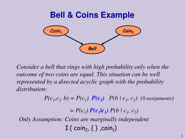
Bell & Coins Example
Bayesian networks provide a powerful tool for modeling diseases, symptoms, and risk factors. These directed acyclic graphs help in understanding the relationships between variables and making probabilistic inferences. By utilizing Bayesian networks, it becomes feasible to represent complex scenarios such as disease manifestations, symptom severity, and the influence of various risk factors in a structured and informative manner.

Download Presentation

Please find below an Image/Link to download the presentation.
The content on the website is provided AS IS for your information and personal use only. It may not be sold, licensed, or shared on other websites without obtaining consent from the author.If you encounter any issues during the download, it is possible that the publisher has removed the file from their server.
You are allowed to download the files provided on this website for personal or commercial use, subject to the condition that they are used lawfully. All files are the property of their respective owners.
The content on the website is provided AS IS for your information and personal use only. It may not be sold, licensed, or shared on other websites without obtaining consent from the author.
E N D
Presentation Transcript
Bell & Coins Example Coin2 Coin1 Bell Consider a bell that rings with high probability only when the outcome of two coins are equal. This situation can be well represented by a directed acyclic graph with the probability distribution: P(c1,c2 b) = P(c1) P(c2) P(b | c1, c2) (8 assignments) = P(c1) P(c2|c1) P(b | c1, c2) Only Assumption: Coins are marginally independent I( coin2, { } ,coin1) 1
Bayesian Networks (Directed Acyclic Graphical Models) Definition: A Bayesian Network is a pair (P,D) where P is a Probability distribution over variables X1 , , Xn and D is a Directed Acyclic Graph (DAG) over vertices X1 , , Xn with the relationship: ? P(x1 , , xn ) = ?=1 P(xi | pai) for all values xi of Xi and where paiis the set of parents of vertex xi in D. (When Xi is a source vertex then paiis the empty set of parents and P(xi | pai) reduces to P(xi).) DAG = directed graph without any directed cycles. 2
Bayesian Networks (BNs) Examples to model diseases & symptoms & risk factors One variable for all diseases (values are diseases) (Draw it) One variable per disease (values are True/False) (Draw it) Na ve Bayesian Networks versus Bipartite BNs (details) Adding Risk Factors (Draw it) 3
Nave Bayes for Diseases & Symptoms D ... sk s2 s1 Values of D are {D1, Dm} and represent non-overlapping diseases. Values of each symptom S represent severity of symptom {0,1,2}. ? P(d, s1 , , sk ) = p(d) ?=1 P(si | d) 4
Risks, Diseases, Symptoms R1 R2 ... D1 D2 D3 Dn ... s3 s2 sk-1 sk s1 Values of each Disease Di are represent existence/non-existence {True, False}. Values of each symptom S represent severity of symptom {0,1,2}. 5
Natural Direction of Information Consider our example of a hypothesis H=h indicating disease and a set of symptoms such as fever, blood pressure, pain, etc, marked by S1=s1, S2=s2, S3=s3 or in short E=e. We assume P(e | h) are given (or inferred from data) and compute P(h | e). Natural order to specify a BN is usually according to causation or time line. Nothing in the definition dictates this choice, but normally more independence assumptions are explicated in the graph via this choice. Example: Atomic clock + watch clocks na ve Bayes model. 6
The Visit-to-Asia Example Visit to Asia Smoking Tuberculosis Lung Cancer Abnormality in Chest Bronchitis Dyspnea X-Ray What are the relevant variables and their dependencies ? 7
An abstract example ) , b P s l P v t = ( , , v , , , , P v s t l b a x d ( ) ( ) ( | ) ( | ) ( | ) ( | , ) ( | ) ( | , ) P P s P s P a t l P x a P d a b In the order V,S,T,L,B,A,X,D, we have a boundary basis: I( S, { }, V ) I( T, V, S) I( l, S, {T,V}) I( X,A, {V,S,T,L,B,D}) S V L T B A X D Does I( {X,D} ,A,V) also hold in P ? 8
Independence in Bayesian networks n = i = i = pa ( , , ) ( | ) (*) p x x p x 1 n i i 1 n = ( , , ) ( | , ) p x x p x x x 1 1 1 n i i 1 I( Xi ,pai , {X1, ,Xi-1} \ pai ) This set of n independence assumptions is called Basis(D) . This equation uses specific topological order d of vertices, namely, that for every Xi, the parents of Xi appear before Xi in this order. However, all choices of a topological order are equivalent. Check for example topological orders of V,S,T,L of visit-to-Asia example. 9
Directed and Undirected Chain Example X2 X3 X4 X1 P(x1,x2,x3,x4) = P(x1) P(x2|x1) P(x3|x2) P(x4|x3) Assumptions: I( X3 ,X2 , X1), I( X4 , X3,{X1, X2}) X2 X3 X4 X1 P(x1,x2,x3,x4) = P(x1, x2) P(x3|x2) P(x4|x3) Markov network: The joint distribution is a Multiplication of functions on three maximal cliques with normalizing factor 1. 10
Reminder: Markov Networks (Undirected Graphical Models) Definition: A Markov Network is a pair (P,G) where P is a probability distribution over variables X1 , , Xn and G is a undirected graph over vertices X1 , , Xn with the relationship: ? P(x1 , , xn ) = K ?=1 gj(Cj ) for all values xi of Xi and where C1 Cm are the maximal cliques of G and gj are functions that assign a non-negative number to every value combination of the variables in Cj. Markov Networks and Bayesian networks represent the same set of independence assumptions only on Chordal graphs (such as chains and trees). 11
From Separation in UGs To d-Separation in DAGs 12
Paths Intuition: dependency must flow along paths in the graph A path is a sequence of neighboring variables S V Examples: X A D B A L S B L T B A X D 13
Path blockage Every path is classified given the evidence: active -- creates a dependency between the end nodes blocked does not create a dependency between the end nodes Evidence means the assignment of a value to a subset of nodes. 14
Path Blockage Blocked Blocked Active Three cases: Common cause S S B L B L 15
Path Blockage Blocked Blocked Active Three cases: Common cause S S L L Intermediate cause A A 16
Path Blockage Blocked Blocked Active Three cases: Common cause T L A Intermediate cause T L X A Common Effect T L X A X 17
Definition of Path Blockage Definition: A path is active, given evidence Z, if Whenever we have the configuration T L A then either A or one of its descendents is in Z No other nodes in the path are in Z. Definition: A path is blocked, given evidence Z, if it is not active. Definition: X is d-separated from Y, given Z, if all paths from a node in X and a node in Y are blocked, given Z. Denoted by ID(X, Z, Y) . (X,Y,Z) are sets of variables that are disjoint. 18
Example ID(T,S| ) = yes S V L T B A X D 19
Example ID (T,S | ) = yes ID(T,S|D) = no S V L T B A X D 20
Example ID (T,S | ) = yes ID(T,S|D) = no ID(T,S|{D,L,B}) = yes S V L T B A X D 21
Example In the order V,S,T,L,B,A,X,D, we get from the boundary basis: ID( S, { }, V ) ID( T, V, S) ID( l, S, {T,V}) ID( X,A, {V,S,T,L,B,D}) S V L T B A X D 22
Main results on d-separation The definition ofID(X, Z, Y) is such that: Soundness [Theorem 9]: ID(X, Z, Y)= yes implies IP(X, Z, Y) follows from Basis(D). Completeness [Theorem 10]: ID(X, Z, Y)= no implies IP(X, Z, Y) does not follow from Basis(D). 23
Revisiting Example II S V L T B A X D So does IP( {X,D} ,A, V)hold ? Enough to check d-separation ! 24
Local distributions- Asymmetric independence Tuberculosis (Yes/No) Lung Cancer (Yes/No) p(A|T,L) Abnormality in Chest (Yes/no) Table: p(A=y|L=n, T=n) = 0.02 p(A=y|L=n, T=y) = 0.60 p(A=y|L=y, T=n) = 0.99 p(A=y|L=y, T=y) = 0.99 Independence for some values IP(A, L=y, T) holds IP(A, L=n, T) does not hold So: IP(A, L, T) does not hold 25
Claim 1: Each vertex Xi in a Bayesian Network is d- separated of all its non-descendants given its parents pai. Proof : Each vertex Xi is connected to its non-descendantsi via its parents or via its descendants. All paths via its parents are blocked because pai are given and all paths via descendants are blocked because they pass through converging edges Z were Z is not given. Hence by definition of d-separation the claim holds: ID(Xi, pai, non-descendantsi). 26
Independence in Bayesian networks n = i = ( , , ) ( | , ) p x x p x x x 1 1 1 n i i 1 = n = i = pa ( , , ) ( | ) (*) p x x p x 1 n i i 1 Implies for every topological order d ? ? ?(? ?(1, ,? ?(? = ?(??(? |???(? ?=1 = ? ?(? ?(1, ,? ?(? = ?(??(? |?d(1 , ??(? 1 ?=1
Claim 2: Each topological order d in a BN entails the same set of independence assumptions. Proof : By Claim 1: ID(Xi, pai, non-descendandsi) holds. For each topological order d on {1, ,n}, it follows IP(Xd(i), pad(i), non-descendsd(i)) holds as well. From soundness (Theorem 9) IP(Xd(i), pad(i), non-descendsd(i)) holds as well. By the decomposition property of conditional independence IP(Xd(i), pad(i), S) holds for every S that is a subset of non-descendsd(i) . Hence, Xi is independent given its parents also from S ={all variables before Xi in an arbitrary topological order d}. 28
Extension of the Markov Chain Property For Markov chains we assume Basis(D): IP(Xi , Xi-1 , {X1 Xi-2}) Due to soundness of d-separation (Theorem 9) we also get: IP(Xi , {Xi-1 ,Xi+1} , {X1 Xi-2 , Xi+2 Xn }) Definition: A Markov blanket of a variable X wrt probability distribution P is a set of variables B(X) such that IP(X, B(X), all-other-variables) Chain Example: B(Xi) = {Xi-1 ,Xi+1}
Markov Blankets in BNs Proof: Consequence of soundness of d-separation (Theorem 9). 30


")