Asymptotic Series: Properties and Notations
Asymptotic series play a crucial role in analyzing functions as their magnitude grows. Explore the properties and notations of asymptotic series, including Big O and Small o notations. Learn how these series show the behavior of functions as their input values increase.

Uploaded on Mar 10, 2025 | 0 Views
Download Presentation

Please find below an Image/Link to download the presentation.
The content on the website is provided AS IS for your information and personal use only. It may not be sold, licensed, or shared on other websites without obtaining consent from the author.If you encounter any issues during the download, it is possible that the publisher has removed the file from their server.
You are allowed to download the files provided on this website for personal or commercial use, subject to the condition that they are used lawfully. All files are the property of their respective owners.
The content on the website is provided AS IS for your information and personal use only. It may not be sold, licensed, or shared on other websites without obtaining consent from the author.
E N D
Presentation Transcript
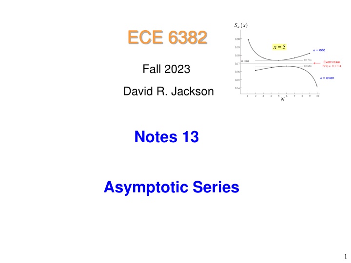
( ) x S N ECE 6382 x = 5 n = odd Exact value F(5) = 0.1704 Fall 2023 n = even David R. Jackson N Notes 13 Asymptotic Series 1
Asymptotic Series An asymptotic series (as z ) is of the form a z ( ) f z z n n as = 0 n or a z a z ( ) f z + + + a 1 2 2 0 Note the asymptotically equal to sign. The asymptotic series shows how the function behaves as z gets large in magnitude. Important point: An asymptotic series does not have to be a converging series. (This is why we do not use an equal sign.) 2
Asymptotic Series (cont.) Properties of an asymptotic series: a z a z ( ) f z + + + a 1 2 2 0 For a fixed number of terms in the series, the series get more accurate as the magnitude of z increases. For a fixed value of z, the series does not necessarily get more accurate as the number of terms increases. The series does not necessarily even converge as we increase the number of terms, for a fixed value of z. ( ) f w + a w a w + + 2 0 a w Note: We can also talk about as 0 1 2 = Use : 1/ w z 3
Big O and Small o Notation This notation is helpful for defining and discussing asymptotic series. Big O notation: ( ) ( ) f z ( ) = O g z Qualitatively, this means that f goes to zero like g as z gets large (or possibly goes to zero even faster than g). Definition: There exists a constant k and a radius R such that ( ) f z ( ) k g z For all z R 4
Big O and Small o Notation (cont.) Examples: 1 1 z 10 z 1 z O = O z 1 z 2 z 1 z + = O 2 1 z 1 z 1 z 1 z 1 1 3! 1 z 1 1 5! 1 1 5! = = sin O + Note: sin 3 5 z z 1 z 1 3! = + 3 2 z 5
Big O and Small o Notation (cont.) Small o notation: ( ) ( ) f z ( ) = o g z Qualitatively, this means that f gets smaller faster than g as z gets large. Definition: For any there exists a radius R (which depends on )such that ( ) f z ( ) g z For all z R 6
Big O and Small o Notation (cont.) Examples: 1 z 1 z 1 z 10 z = o o 2 1 z 3 z 1 z + = o 2 3 1 m z ( ) z = = z , 1,2,3, arg e o m 2 2 = = cos sin z x iy r ir Note: e e e e e 7
Big O and Small o Notation (cont.) Note: ( ) ( ) ( ) f z ( ) ( ) f z ( ) = = o g z O g z ( ) ( ) ( ) f z ( ) ( ) f z ( ) = = O g z o g z Examples: 1 z 1 z 1 z 1 z = = o O 2 2 5 z 1 z 5 z 1 z = = O o 8
Definition of Asymptotic Series a z ( ) f z z n n as = 0 n Definition of asymptotic series: In order to have an asymptotic series we require the following: a z 1 N z N ( ) f z = n n o For any N = 0 n As z gets large, the error in stopping at term n = Ngets smaller than the last term in the series. a z a z a z ( ) f z + + + + a 1 2 2 3 3 Example: 0 This ensures that the last term kept is meaningful. 1 z a z a z ( ) f z + + = a o 1 2 2 0 2 9
Theorem for Asymptotic Series Theorem a z ( ) f z z n n as If = 0 n N 1 N a z ( ) f z = O N n n Then for any + 1 z = 0 n Note: 1 N 1 N z 1 N + O o + 1 z 1 N z o O Example: 1 z 1 z a z a z ( ) f z + + = a 1 2 2 O 0 3 10
Theorem for Asymptotic Series (cont.) Proof of theorem a z ( ) f z z n n as Assume = 0 n + 1 N 1 N a z ( ) f z = o n n (from definition of asymptotic series) + 1 z = 0 n a z a z 1 N N ( ) f z = + + 1 1 n n N N o + 1 z = 0 n N 1 N 1 N a z a z ( ) f z = + = + + o O 1 1 n n N N + + 1 1 z z = 0 n 11
Summing Asymptotic Series One must be careful when summing an asymptotic series, since it may diverge: it is not clear what the optimum number of terms is, for a given value of z= z0. N a z ( ) f z ? N n n What is the optimum 0 = 0 n 0 General rule of thumb : Pick N so that the N+1 term in the series is the smallest. (See the example later.) 12
Summing Asymptotic Series (cont.) Rule of Thumb Principle: As x gets large, the error in stopping with term N is approximately given by thefirst term that is omitted (i.e., the N+1 term). To see this, use: + 1 N a z 1 N ( ) f z = n n o (from definition of asymptotic series) + 1 z = 0 n Therefore, we have (separating out the last term from the sum) 1 N a z a z N ( ) f z = + + + + 1 1 n n N N o + 1 z = 0 n This is an asymptotic estimate of the error. Hence: a z a z N ( ) N ( ) f z = + + Error 1 1 n n N N = 0 n 13
Generation of Asymptotic Series Various method can be used to generate an asymptotic series expansion of a function: Integration by parts* The method of steepest descent Watson s lemma Other specialized techniques * This method is discussed in this set of notes. 14
Example The exponential integral function (of order 1): t e ( ) , . E z dt path does not cross the real axis C 1 t z ( ) Im t ( ) Im z z Branch cut z ( ) ( ) Re t Re z X Note: z The branch cut is not arbitrary here. Note:E1 (z) is discontinuous (by 2 i) across the negative real axis: t e ( ) ( ) ( ) a i a i + = = 2 Res 2 0, 0 E E i i a 1 1 t = 0 t 15
Example (cont.) b b dv dt du dt b = Use integration by parts: u dt uv vdt a a a t 1 t e ( ) = t E z dt e dt Note: 1 t d v t z z It is very important which of the two functions is chosen to be u and which one is chosen to be v. u d 1 t 1 t ( ) ( ) = t t e e dt 2 z z z 1 t e = t e dt 2 z z z 1 t 2 e ( ) ( ) = t t e e dt 2 3 z t z z z z 2 t e e z = + t e dt 2 3 z z 16
Example (cont.) Using integration by parts N times: Error term z z z 1 N e e z e z ( ) z ( ) ( ) ( ) 1 N N = + + + tt 1 1 ! 1 ! E N N e d 1 + 2 1 N z t z or ( ) ( N ) 1 N 1 1 ! N 1 z 1 z 1 N ( ) z ( ) N = + + + z t 1 ! E e N e d t 1 + 2 1 z t z Question: Is this a valid asymptotic series: ( ) ( n ) 1 n 1 1 ! n ( ) f z ( ) z ??? e E z Note:a0 = 0 here. 1 z = 1 n 17
Example (cont.) Examine the difference term: ( ) ( N ) 1 N 1 1 ! N 1 z 1 z 1 N ( ) ( ) N + + = z z t 1 ! e E z e N e dt 1 N + 2 1 z t z 1 N 1 N = z t z z ! ! e N e dt e N e + + N 1 1 z z z or 1 N = = z z z z Note: 1 e e e e ! N + N 1 z so 1 N 1 N z = = O o N + 1 z 18
Example (cont.) Hence, we have: ( ) ( n ) 1 n 1 1 ! n 1 z 1 z 2 z 6 z 24 z 120 z ( ) f z ( ) = + + + z e E z 1 2 3 4 5 6 z = 1 n ( ) ( n ) 1 n 1 1 ! n a z = = b n n b Question: Is this a converging series? n n z 1 n Use the d Alembert ratio test: n ! z n = lim n L ( ) + 1 n 1 ! z n b = + lim n 1 n L 1 z b ( ) n = = lim n n 1: 1: L L converges diverges The series diverges! 19
Example (cont.) x = 5 ( ) ( n ) 1 n n 1 2 3 4 5 6 7 8 9 bn 0.2 -0.04 0.016 -0.00916 0.00768 -0.00768 0.00922 -0.013 0.021 -0.037 1 1 ! n ( ) ( n ) 1 n ( ) f x ( ) 1 1 ! n a x x e E x = b n n 1 n x x = 1 n ( ) x ( ) ( n ) 1 n S 1 1 ! n N N ( ) x = N S b N n x = = 1 1 n n N = 1 x = 5 n= odd N = 7 N = 5 N = 3 Exact value f(5) = 0.1704 N = 6 10 N = 4 N = 2 N = 8 n= even Using n = 5 or 6 is optimum for x = 5. This is also where |bn| is the smallest. N 20
Example (cont.) t e ( ) f x ( ) = x x e E x e dt 1 t x Exact function 2 1.76 1.5 ( ) f x F x ( ) 1 0.5 0.092 0 0 0 2 4 6 8 10 xx 10 21
Example (cont.) ( ) ( n ) 1 n 1 1 ! n N ( ) x ( ) f x Error N x = 1 n Exact error 1.0 1 0.2 0.1 0.1 ( ) ErrorNx , Error 1 x ( ) N = 1 , Error 2 x ( ) 0.01 0.01 , Error 3 x ( ) N = 2 0.001 3 1 10 N = 3 0.0001 0.0001 4 1 10 0 0.015 5 10 10 15 0 5 15 xx 15.001 22
Example (cont.) ( ) ( n ) 1 n ( ) N N 1 1 ! n N 1 x ! N ( ) x ( ) f x Error AsyError N N + 1 x = 1 n 1.0 Solid: actual error Dashed: asymptotic error estimate ( ) ErrorNx 0.1 ( ) AsyErrorNx N = 1 0.01 N = 2 0.001 x 23
Note on Converging Series Assume that a series converges for all |z|>R (for some R), so that a z = ( ) f z n n = 0 n Then it must also be a valid asymptotic series: a z = ( ) f z n n 0 n Proof: N N 1 N a z a z a z a ( ) f z = + = + + + + a 2 n n n n n n N z + 1 N + 1 z = n N = + = 0 1 0 n n ( ) N Is this 1 / ? o z 24
Note on Converging Series (cont.) N 1 N a z a ( ) f z = + + + + a 2 n n N z + 1 N + 1 z = 0 n Converging series We note that a + + + a a z 2 N z as + + 1 1 N N 1 N 1 N 1 z a + + = = + 2 N z a O o + 1 N + + 1 1 N z z 25
Note on Converging Series (cont.) Example: 1 z 1 1 2! 1 1 3! = + + + + 1/ z 1 e 2 3 z z The point z = 0 is an isolated essential singularity, and there are no other singularities out to infinity. This Laurent series converges for all z 0 (hence for |z| > R). This is a valid asymptotic series. 1 z 1 1 2! 1 1 3! + + + + 1/ z 1 e 2 3 z z 26
Stationary-Phase Method The stationary phase method is sometimes useful for getting the leading term of the asymptotic series for integrals of this form: b ( ) f x e ( ) = ( ) g x i I dx a Note: The integral must be along the real axis. Assumption: There is a stationary phase point inside the integration interval.: ( ) ( ) g x = 0 , x a b 0 0 27
Stationary-Phase Method (cont.) ( ) ( ) a b = ( ) g x i I f x e dx ( ) ( ) g x = 0 , x a b (stationary phase point) 0 0 ( ) f x ( ) x Assume 0, 0 g 0 0 1 2 ( ) ( ) g x ( )( 0 g x ) ( )( 0 x ) 2 + + g x x x g x x 0 0 0 ( ) ( ) f x = ( ) g x j Re f x e ( ) ( ) Stationary-phase point g x cos x 0x b a 28
Stationary-Phase Method (cont.) Assumption: + x i g x 0 ( ) ~ ( ) f x e I dx x 0 If 0 ( ) slowenough ) 1 ( (This is justified a little later.) 29
Stationary-Phase Method (cont.) + x i g x 0 ( ) ~ ( ) f x e I dx x 0 Since 0 ( ) f x ( ) f x 0 Hence + x i g x 0 ( ) ~ ( ) f x I e dx 0 x 0 30
Stationary-Phase Method (cont.) + x i g x 0 ( ) ~ ( ) f x I e dx 0 x 0 1 2 ( ) ( ) g x ( )( 0 g x ) ( )( 0 x ) 2 + + g x x x g x x 0 0 0 so 1 2 ( )2 + x x ( ) x i g x ( ) ( ) f x e i g x ( ) 0 0 0 I e dx 0 0 x 0 or 1 2 ( )2 + x x ( ) x i g x ( ) ( ) f x e ( ) 0 0 0 i g x I e dx 0 0 x 0 where ( ) x ( ) x = g g 0 0 31
Stationary-Phase Method (cont.) Let ( ) 2 ( ) 2 g x g x ( ) 0 0 = = ds dx s x x 0 Then 2 + S ( ) ( ) f x e 2 i g x ( ) L is I e ds 0 ( ) x 0 g S L 0 where ( ) 2 g x 0 = S L , S As if L 32
Stationary-Phase Method (cont.) Therefore ( ) + + S 2 2 L is is I e ds e ds L S L Let + 2 2 + + + = is is I e ds e ds L C (We can change the path by Cauchy s theorem.) ( ) Im s C 45 ( ) Re s C 33
Stationary-Phase Method (cont.) + 2 2 + + + = is is I e ds e ds L C Let i = = 2 2 2 s t e it 2 i = s te 4 i = ds dte 4 Hence Similarly, ( ) + 2 j i it + + = I e e dt 2 4 is I e ds L L + i 2 i = t e e dt 4 = e 4 i = e 4 34
Stationary-Phase Method (cont.) b ( ) f x e ( ) = ( ) g x i I dx a Final result: Then 2 i ( ) i g x ( ) f x e I e 4 0 ( ) x 0 g 0 ( ) ( ) x + , 0 g x 0 , 0 g 0 O 1 = Note: I 35
Example 1 ( ) x ( ) = cos sin J x d 0 0 This is an integral form of the Bessel function of the first kind of order zero. We want to evaluateJ0(x) for large x. (We let x be called .) 1 ( ) = ( ) cos sin J d 0 0 36
Example (cont.) 1 ( ) = ( ) cos sin J d 0 0 1Re = sin i e d 0 ( ) ( ) ( ) = = 1 f sin g ( ) g = = cos 0 0 0 = +n 0 2 37
Example (cont.) Stationary-phase point / 2 / 2 ( ) ( ) ( ) ( ) g = = = sin = = g sin 1 0 0 cos g ( ) g = = sin 1 0 0 0 sin g Hence, we have: 1 2 i ( ) ( ) 1 i ~ Re J e e 4 0 1 Note: In the final result we can relabel x. 38
Example (cont.) Hence, the final result is: 2 ( ) x ~ cos J x 0 4 x as x 39
")

")

")
")
")
")


")

")


")
")
")
")
")
")
")
")

")
")

")
")
")
")
")
")
")
")

")
")
")