Analyzing Interpolation and Extrapolation Techniques
Explore polynomial interpolation, Vandermonde matrix equations, condition numbers, proofs, norms, vector and matrix norms, and commonly used norms in mathematics. Understand the concepts and applications of interpolation and extrapolation through detailed explanations and visual aids.

Download Presentation

Please find below an Image/Link to download the presentation.
The content on the website is provided AS IS for your information and personal use only. It may not be sold, licensed, or shared on other websites without obtaining consent from the author.If you encounter any issues during the download, it is possible that the publisher has removed the file from their server.
You are allowed to download the files provided on this website for personal or commercial use, subject to the condition that they are used lawfully. All files are the property of their respective owners.
The content on the website is provided AS IS for your information and personal use only. It may not be sold, licensed, or shared on other websites without obtaining consent from the author.
E N D
Presentation Transcript
Chapter 3, Interpolation and Extrapolation
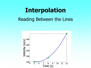
Interpolation & Extrapolation (xi,yi) Fit an analytic function f(x) that passes through the given N points exactly.
Polynomial Interpolation Use polynomial of degree N-1 to fit exactly N data points (xi,yi), i =1, 2, , N. ( ) f x c c x c x = + + + + 2 1 N c x 0 1 2 1 N The coefficients ci are determined by a system of linear equations, such that ? ?? = ??, ? = 1,2, ,?.
Vandermonde Matrix Equation 2 1 2 2 1 N c c y y 1 1 x x x x x x 0 1 1 1 1 N 1 2 = 2 2 2 N 1 N N c y 1 x x x 1 N N N But it is not advisable to solve this system numerically because of possible ill- conditioning.
Condition Number cond(A) = ||A|| ||A-1|| For singular matrix, cond(A) = A linear system is ill-conditioned if cond(A) is very large. Stability of linear system Ax=b: ?? ? ?? ? ?? ? cond ? +
Prove: ? = ? 1?,?? = ?? 1? + ? 1?? (Leiniz rule) ?? 1? + | ? 1?? | (triangle ineq) ?? 1= 1, ?? 1= ? 1??? 1 ?? = ? means ? ? ?? ? 1??? 1? / ? + | ? 1?? |/ ? ?? ? ? ? ? 1?? + ? 1?? / ? ?? ?? ? 1 ? + ? ?
Definition of norm Norm || . ||: a real function that satisfies (1) f(A) > 0, if A 0, (2) f(A+B) f(A) + f(B), (3) f( A) = | | f(A). With norm, we can talk about error, limit, convergence, continuity, etc, in vector space or matrices.
Norms Vector p-norm (p 1) ( | = p x x ) 1/ p + + p p p | | | | | x x 1 2 N Induced matrix norm || || Ax = sup x A || || x 0 ?? ? ? ?? ? ? sup: supremum (or least upper bound)
Commonly Used Norms Vector norm N N = = 2 j || x || | x |, || x || x 1 j 2 = = j 1 j 1 = || x || max | j x | j Matrix norm N i N Where is the maximum eigenvalue of matrix ATA. = = || A || max j | a |, || A || 1 ij 2 = j 1 = || A || max i | a | ij = 1
Lagranges Formula It can be verified that the solution to the Vandermonde equation is given by the formula below: N ( ) x x j N = , 1 j i j N = = ( ) f x ( ) , l x y ( ) l x i i i = 1 i ( ) x x i j j i j = , 1 li(x) has the property li(xj) = ij.
l1(x) for xi = 0, 1, 3 The Lagrange basis polynomial li(x) is defined by the property: li(xj) = ij
Joseph-Louis Lagrange (1736-1813) Italian-French mathematician associated with many classic mathematics and physics Lagrange multipliers in minimization of a function, Lagrange s interpolation formula, Lagrange s theorem in group theory and number theory, and the Lagrangian (L=T-V) in mechanics and Euler-Lagrange equations.
Nevilles Algorithm Evaluate Lagrange s interpolation formula f(x) at a given point x, from the data points (xi,yi). Interpolation tableau P x1: y1 = P1 P12 x2: y2 = P2P123 P23P1234 x3: y3 = P3P234 P34 x4: y4 = P4 Pi,i+1,i+2, ,i+n is a polynomial of degree n in x that passes through the points (xi,yi), (xi+1,yi+1), , (xi+n,yi+n) exactly.
Determine P12 from P1 & P2 Given the value P1 and P2 at x=x1 and x2, we find linear interpolation P12(x) = (x) P1+[1- (x)] P2 Since P12(x1) = P1 and P12(x2) = P2, we must have (x1) = 1, (x2) = 0 so (x) = 12= (x-x2)/(x1-x2)
Determine P123 from P12 & P23 We write P123(x) = (x) P12(x) + [1- (x)] P23(x) P123(x2) = P2 already for any choice of (x). We require that P123(x1)=P12(x1) =P1 and P123(x3)=P23(x3) =P3, thus (x1) = 1, (x3) = 0 or = = x x x x ( ) x 3 13 1 3
Recursion Relation for P Given two m-point interpolated value P constructed from point i,i+1,i+2, ,i+m-1, and i+1,i+2, ,i+m, the next level m+1 point interpolation from i to i+m is a linear combination: ( ) = ( ) x P + ( ) x P 1 P 1)( + + i m + 1)...( + + 1)( + + i m + ( 2)...( ) ( 1) ( 2)...( ) i i i i i i m x x i i i m x x = ( )( i i m = + where ( ) x + ) i m + i
Evaluate f(3) given 4-points (0,1), (1,2), (2,3),(4,0), us P table. = + (1 ) P P x x P i m + + 1, , + i m + , , , , 1 i i i m x x i x1=0, y1=1 =P1 ( )( i i m = i m + + ) P1,2 = 4 ? = 2 i m + i ? = 1 P1,2,3 = 4 x2=1, y2=2 =P2 2 P2,3 = 4 ? =1 ? = 1 P1,2,3,4= 11/4 4 ? =1 x3=2, y3=3 =P3 P2,3,4 = 7/3 3 P3,4 = 3/2 ? =1 2 x4=4, y4=0 =P4
Use Small Difference C & D P1 C1,1 = P12-P1 ( )( x ) x x C D + , 1 m i x + + , = i m i C P12 + 1, m i 1 i i m D1,1 C2,1=P123-P12 P123 P2 D2,1 C1,2 C3,1=P1234-P123 P23 P1234 D1,2 C2,2 P234 D3,1=P1234-P234 P3 C1,3 D2,2=P234-P34 P34 ( )( ) i m x + + x C D D1,3 + 1 , 1 m i , = m i D + 1, m i x i m x + + P4 1 i
Deriving the Relation among C & D PA D1=PA P0 C2=P-PA P0 P = PA + (1- )PB C1=PB P0 D2=P-PB PB = = = = = ) ) ( C P P P P P ( P P P ) = D ( C D ) 2 A 0 A 0 2 1 1 (1 + + P P (1 P C P P ) A B 0 A P 0 )( ( P ) (1 D )( ) ( P P ) A 0 B 0 A 0 1 1
Evaluate f(3) given 4-points (0,1), (1,2), (2,3),(4,0). = (1 )( ) C , 1 m i C D C0,1=1 + + + + 1, ( )( i i m x x 1) , m i m i x1=0, y1=1 =P1 C1,1 = 3 x x ( )( i i m = i m + + 1 D0,1=1 + + 1) i m + + 1 i C2,1= 0 D1,1= 2 C0,2=2 x2=1, y2=2 =P2 C1,2= 2 C3,1= - 5/4 D2,1= 0 D0,2=2 P1234= 11/4 D1,2= 1 C2,2= -5/3 C0,3=3 D3,1=5/12 x3=2, y3=3 =P3 C1,3= -3/2 D2,2=5/6 D0,3=3 D1,3 = 3/2 = ( )( i i m ( ) D , 1 m i C D C0,4=0 + + + + 1, 1) , m i m i x4=4, y4=0 =P4 D0,4=0
polint( ) Program import math def polint(xa, ya, n, x, y, dy): c = ya.copy() d = ya.copy() ns = 0 dif = math.fabs(x-xa[0]) for i in range(1,n): dift = math.fabs(x-xa[i]) if (dift < dif): ns = i dif = dift y[0] = ya[ns] ns -= 1
polint(), continued for m in range(1,n): for i in range(0,n-m): ho = xa[i]-x hp = xa[i+m]-x w = c[i+1]-d[i] den = ho hp den = w/den d[i] = hp*den c[i] = ho*den if(2*(ns+1) < (n-m)): dy[0] = c[ns+1] else: dy[0] = d[ns] ns -= 1 y[0] += dy[0]
Piecewise Linear Interpolation x x x x ( ) = ( ) x y + = ( ) 1 ( ) x , ( ) x 2 P x y 12 1 2 y 1 2 P23(x) P12(x) (x3,y3) (x2,y2) P34(x) (x4,y4) (x1,y1) P45(x) (x5,y5) x
Piecewise Polynomial Interpolation y Discontinuous derivatives across segment P1234(x) P1234(x) (x3,y3) (x2,y2) P2345(x) (x4,y4) (x1,y1) P2345(x) (x5,y5) x
Cubic Spline, Pi(x) is cubic Same 1st and 2nd derivatives at the connection point. y P2(x) P1(x) P3(x) (x3,y3) (x2,y2) P4(x) (x1,y1) (x4,y4) (x5,y5) x ??? = ???3+ ???2+ ??? + ??, ? = 1,2,3,4
Cubic Spline Given N points (xi,yi), i=1,2, ,N, for each interval between points i to i+1, fit to cubic polynomials such that Pi(xi)=yi and Pi(xi+1)=yi+1. Make 1st and 2nd derivatives continuous across intervals, i.e., Pi(n)(xi+1) = P(n)i+1(xi+1), n = 1 and 2. Fix boundary condition to P(2)(x1 or N)=0, to completely specify.
Reading NR, Chapter 3 See also J. Stoer and R. Bulirsch, Introduction to Numerical Analysis, Chapter 2.
Problems for week 4/ch 3 (Interpolation) due 19 Sep 2024 1. Use Neville s algorithm by hand to find the interpolation value at x = 0, for a cubic polynomial interpolation with 4 points (x,y) = (-1,1.25), (1,2), (2,3), (4,0). Give the P table as well as C/D table. Also write out the Lagrange s formula and then evaluate f(0). 2. Given the same 4 points as above, determine the cubic splines with natural boundary condition (second derivatives equal to 0 at the boundaries). Use a direct fit to the three cubic polynomials. Solve the 12 12 linear system by the code ludcmp.py. Give the cubic polynomials numerically in each of the three intervals.


 for xi = 0, 1, 3")
")


 given 4-points (0,1), (1,2),")


 given 4-points (0,1), (1,2),")
 Program")
, continued")


 is cubic")


")