Analyzing Categorical Data and Chi-Square Test
Categorical data analysis, contingency tables, chi-square test, likelihood ratio, odds ratio, and loglinear models are vital in statistics. Understanding the theory, assumptions, and interpretation of these methods is crucial for drawing meaningful conclusions from categorical data. Explore examples of data consisting of unique categories and learn how to analyze frequencies using contingency tables. Dive into an example involving dancing cats and dogs to understand how to analyze two or more categorical variables. Discover how Pearsons Chi-Square Test can help determine relationships between different categorical variables.

Download Presentation

Please find below an Image/Link to download the presentation.
The content on the website is provided AS IS for your information and personal use only. It may not be sold, licensed, or shared on other websites without obtaining consent from the author.If you encounter any issues during the download, it is possible that the publisher has removed the file from their server.
You are allowed to download the files provided on this website for personal or commercial use, subject to the condition that they are used lawfully. All files are the property of their respective owners.
The content on the website is provided AS IS for your information and personal use only. It may not be sold, licensed, or shared on other websites without obtaining consent from the author.
E N D
Presentation Transcript
Categorical Data Prof. Andy Field
Aims Categorical data Contingency tables chi-square test Likelihood ratio Odds ratio Loglinear models Theory Assumptions Interpretation Slide 2
Categorical Data Sometimes we have data consisting of the frequency of cases falling into unique categories Examples: Number of people voting for different politicians Numbers of students who pass or fail their degree in different subject areas Number of patients or waiting list controls who are free from diagnosis (or not) following a treatment Slide 3
An Example: Dancing Cats and Dogs Analysing two or more categorical variables The mean of a categorical variable is meaningless The numeric values you attach to different categories are arbitrary The mean of those numeric values will depend on how many members each category has. Therefore, we analyse frequencies An example Can animals be trained to line-dance with different rewards? Participants: 200 cats Training The animal was trained using either food or affection, not both) Dance The animal either learnt to line-dance or it did not Outcome: The number of animals (frequency) that could dance or not in each reward condition We can tabulate these frequencies in a contingency table
Pearsons Chi-Square Test Use to see whether there s a relationship between two categorical variables Compares the frequencies you observe in certain categories to the frequencies you might expect to get in those categories by chance. The equation: ( Model ) 2 Observed - Model ij ij 2 = ij i represents the rows in the contingency table and j represents the columns. The observed data are the frequencies the contingency table The model is based on expected frequencies . Calculated for each of the cells in the contingency table. n is the total number of observations (in this case 200). Row Total Column Total i j = = Model E ij ij n Test statistic Checked against a distribution with (r 1)(c 1) degrees of freedom. If significant then there is a significant association between the categorical variables in the population. The test distribution is approximate so in small samples use Fisher s exact test.
Pearsons Chi-Square Test RT CT n 76 38 = = = Yes Food Model 14 44 . Food, Yes 200 RT CT n 124 38 = = = No Food Model 23 56 . Food, No 200 RT CT n 76 162 = = = Yes Affection Model 61 56 . Affection, Yes 200 RT CT n 124 162 = = = No Affection Model 100 44 . Affection, No 200
Likelihood Ratio Statistic An alternative to Pearson s chi-square, based on maximum-likelihood theory. Create a model for which the probability of obtaining the observed set of data is maximized This model is compared to the probability of obtaining those data under the null hypothesis The resulting statistic compares observed frequencies with those predicted by the model i and j are the rows and columns of the contingency table and ln is the natural logarithm Observed ij 2 = L 2 Observed ln ij Model ij Test statistic Has a chi-square distribution with (r 1)(c 1) degrees of freedom. Preferred to the Pearson s chi-square when samples are small.
Likelihood Ratio Statistic 28 10 48 114 L = + + + 2 2 28 ln 10 ln 48 ln 114 ln 14.44 23.56 + 61.56 100.44 ( 18 ) ( 57 . 8 ) ( 44 . 14 ) ( + ) = . 0 + . 0 . 0 2 28 662 10 . 0 + 857 48 249 114 127 = 2 54 . 11 94 . = 24 94 .
Interpreting Chi-Square The test statistic gives an overall result. We can break this result down using standardized residuals. There are two important things about these standardized residuals: Standardized residuals have a direct relationship with the test statistic (they are a standardized version of the difference between observed and expected frequencies). These standardized are z-scores (e.g. if the value lies outside of the range between 1.96 and +1.96 then it is significant at p < .05). Effect Size The odds ratio can be used as an effect size measure.
Important Points The chi-square test has two important assumptions: Independence: Each person, item or entity contributes to only one cell of the contingency table. The expected frequencies should be greater than 5. In larger contingency tables up to 20% of expected frequencies can be below 5, but there a loss of statistical power. Even in larger contingency tables no expected frequencies should be below 1. If you find yourself in this situation consider using Fisher s exact test. Proportionately small differences in cell frequencies can result in statistically significant associations between variables if the sample is large enough Look at row and column percentagesto interpret effects.
Entering Data: the Contingency Table food <- c(10, 28) affection <- c(114, 48) catsTable <- cbind(food, affection) The resulting data look like this:
Running the Analysis with R Commander
The Chi-square Test Using R Commander
Running the Analysis using R For raw data, the function takes the basic form: CrossTable(predictor, outcome, fisher = TRUE, chisq = TRUE, expected = TRUE, sresid = TRUE, format = "SAS"/"SPSS") and for a contingency table: CrossTable(contingencyTable, fisher = TRUE, chisq = TRUE, expected = TRUE, sresid = TRUE, format = "SAS"/"SPSS")
Running the Analysis using R To run the chi-square test on our cat data, we could execute CrossTable(catsData$Training, catsData$Dance, fisher = TRUE, chisq = TRUE, expected = TRUE, sresid = TRUE, format = "SPSS") on the raw scores (i.e., the catsData dataframe), or CrossTable(catsTable, fisher = TRUE, chisq = TRUE, expected = TRUE, sresid = TRUE, format = "SPSS")
Output from the CrossTable() Function
The Odds Ratio danced and food had that Number = Odds dancing after food Number that had food but didn' dance t 28 = 10 = 8 . 2 Number affection had that danced and = Odds dancing affection after Number affection had that but didn' dance t 48 = 114 = . 0 421 Odds dancing after food = Odds Ratio Odds dancing affection after 8 . 2 = . 0 421 = . 6 65
Interpretation There was a significant association between the type of training and whether or not cats would dance 2(1) = 25.36, p < .001. This seems to represent the fact that, based on the odds ratio, the odds of cats dancing were 6.58 (2.84, 16.43) times higher if they were trained with food than if trained with affection.
Loglinear Analysis When? To look for associations between three or more categorical variables Example: dancing dogs Same example as before but with data from 70 dogs. Animal Dog or cat Training Food as reward or affection as reward Dance Did they dance or not? Outcome: Frequency of animals
Theory Our model has three predictors and their associated interactions: Animal, Training, Dance, Animal Training, Animal Dance, Dance Training, Animal Training Dance Such a linear model can be expressed as: ( i b b b b + + + = C B A Outcome 3 2 1 0 ) + + + + + AB AC BC ABC b b b b 4 5 6 7 i A loglinear Model can also be expressed like this, but the outcome is a log value: ( ) ( b b b b b AB C B A O ln 4 k 3 j 2 i 1 0 ijk + + + + = ) ( ) ln + + + + AC BC ABC b b b ij 5 6 7 ik jk ijk ijk
Backward Elimination Begins by including all terms: Animal, Training, Dance, Animal Training, Animal Dance, Dance Training, Animal Training Dance Remove a term and compares the new model with the one in which the term was present: Starts with the highest-order interaction. Uses the likelihood ratio to compare models: 2 Change L = 2 Current L 2 Previous L Model Model If the new model is no worse than the old, then the term is removed and the next highest-order interactions are examined, and so on.
Assumptions Independence An entity should fall into only one cell of the contingency table. Expected frequencies It s all right to have up to 20% of cells with expected frequencies less than 5; however, all cells must have expected frequencies greater than 1. If this assumption is broken the result is a radical reduction in test power. Remedies for problems with expected frequencies: Collapse the data across one of the variables: The highest-order interaction should be non-significant. At least one of the lower-order interaction terms involving the variable to be deleted should be non-significant. Collapse levels of one of the variables: Only if it makes theoretical sense. Collect more data. Accept the loss of power (not really an option given how drastic the loss is).
Loglinear Analysis Using R Data are entered for loglinear analysis in the same way as for the chi-square test. To create the separate dataframes for cats and dogs, we execute: justCats = subset(catsDogs, Animal=="Cat") justDogs = subset(catsDogs, Animal=="Dog") Having created these two new dataframes, we can use the CrossTable() command to generate contingency tables for each of them by executing: CrossTable(justCats$Training, justCats$Dance, sresid = TRUE, prop.t = FALSE, prop.c = FALSE, prop.chisq = FALSE, format = "SPSS") CrossTable(justDogs$Training, justDogs$Dance, sresid = TRUE, prop.t = FALSE, prop.c = FALSE, prop.chisq = FALSE, format = "SPSS")
Loglinear Analysis as a Chi-Square Test The first stage, is to create a contingency table to put into the loglm() function; we can do this using the xtabs() function: catTable<-xtabs(~ Training + Dance, data = justCats) We input this object into loglm().
Loglinear Analysis as a Chi-Square Test Model 1: catSaturated<-loglm(~ Training + Dance + Training:Dance, data = catTable, fit = TRUE) Model 2: catNoInteraction<-loglm(~ Training + Dance, data = catTable, fit = TRUE)
Mosaic Plot To do a mosaic plot in R, we can use the mosaicplot() function: mosaicplot(catSaturated$fit, shade = TRUE, main = "Cats: Saturated Model")
Output from Loglinear Analysis as a Chi-Square Test Output of the saturated model:
Output from Loglinear Analysis as a Chi-Square Test Output of the model without the interaction term
Cats: Saturated Model Affection as Reward Food as Reward >4 2:4 0:2 No -2:0 Dance -4:-2 <-4 Standardized Yes Residuals: Training
Cats: Expected Values Affection as Reward Food as Reward >4 2:4 No 0:2 -2:0 Dance -4:-2 <-4 Yes Standardized Residuals: Training
Loglinear Analysis First of all we need to generate our contingency table using xtabs() and we can do this by executing: CatDogContingencyTable<-xtabs(~ Animal + Training + Dance, data = catsDogs) We start by estimating the saturated model, which we know will fit the data perfectly with a chi-square equal to zero. We ll call the model caturated. We can create this model in the same way as before: caturated<-loglm(~ Animal*Training*Dance, data = CatDogContingencyTable)
Loglinear Analysis: the Saturated Model summary(caturated)
Loglinear Analysis: Model without Three-Way Interaction Next we ll fit the model with all of the main effects and two way interactions: threeWay<-update(caturated, .~. - Animal:Training:Dance) summary(threeWay)
Loglinear Analysis: Comparing Models anova(caturated, threeWay)
Interpreting the Three-Way Interaction The next step is to try to interpret the three-way interaction. We can obtain a mosaic plot by using the mosaicplot() function and applying it to our contingency table: mosaicplot(CatDogContingencyTable, shade = TRUE, main = "Cats and Dogs")
Cats and Dogs Dog Cat No Yes No Yes >4 2:4 Affection as Reward 0:2 -2:0 Training -4:-2 <-4 Standardized Food as Reward Residuals: Animal
Following up with Chi-Square Tests An alternative way to interpret a three-way interaction is to conduct chi-square analysis at different levels of one of your variables. For example, to interpret our animal training dance interaction, we could perform a chi- square test on training and dance but do this separately for dogs and cats. In fact the analysis for cats will be the same as the example we used for chi-square. You can then compare the results in the different animals.
The Odds Ratio for Dogs = Odds Number tha danced and food had t dancing after food Number tha had t food but didn' dance t 20 = 14 = . 1 43 = Odds Number tha affection had t danced and dancing after affection Number tha affection had t but didn' dance t 29 = 7 = . 4 14 Odds = Odds Ratio dancing after food Odds dancing after affection . 1 43 = . 4 14 = . 0 35
Interpretation The three-way loglinear analysis produced a final model that retained all effects. The likelihood ratio of this model was 2 (0) = 0, p = 1. This indicated that the highest-order interaction (the animal training dance interaction) was significant, 2 (1) = 20.31, p < .001. To break down this effect, separate chi-square tests on the training and dance variables were performed separately for dogs and cats. For cats, there was a significant association between the type of training and whether or not cats would dance, 2 (1) = 25.36, p < .001; this was true in dogs also, 2 (1) = 3.93, p < .05. Odds ratios indicated that the odds of dancing were 6.58 higher after food than after affection in cats, but only 0.35 in dogs (i.e., in dogs, the odds of dancing were 2.90 times lower if trained with food compared to affection). Therefore, the analysis seems to reveal a fundamental difference between dogs and cats: cats are more likely to dance for food rather than affection, whereas dogs are more likely to dance for affection than food.
To Sum Up We approach categorical data in much the same way as any other kind of data: We fit a model, we calculate the deviation between our model and the observed data, and we use that to evaluate the model we ve fitted. We fit a linear model. Two categorical variables Pearson s chi-square test Likelihood ratio test Three or more categorical variables Loglinear model For every variable we get a main effect We also get interactions between all combinations of variables Loglinear analysis evaluates these effects hierarchically Effect sizes The odds ratio is a useful measure of the size of effect for categorical data Slide 47


")
")