A Quick Puzzle for Jim Propp's 64th Celebration
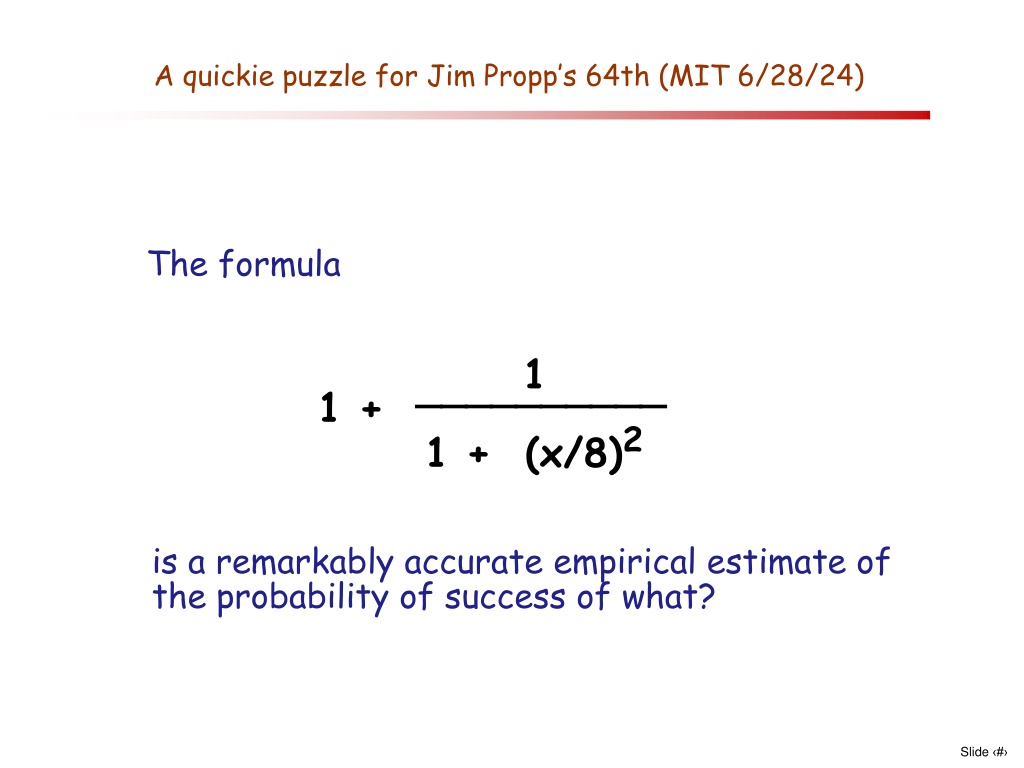


The formula
A quickie puzzle for Jim Propp’s 64th (MIT 6/28/24)

is a remarkably accurate empirical estimate of
the probability of success of what?
A blob begins as a disk of radius 1 on the plane
and grows in all directions at rate
1
.
An unsolved puzzle for Jim Propp’s 64th (MIT 6/28/24)
It can be stopped only by a special kind of
fence that can be built (anywhere) but at total
rate only
λ
.
What is the critical value of
λ
above which the
blob can be surrounded and the world saved,
but below which we are all doomed?

Peter Winkler
with:
Ioana Dumitriu
and
Prasad Tetali
but the real heroes are
John Gittins
and
Richard Weber
Changing Horses among Markov Chains
In honor of Jim Propp’s 64th and the Whirling Tour (MIT 6/29/24)
First: the Whirling Tour
You have a tree (perhaps with some loops); you start
at vertex
u
and want to walk to
v
.
Thm.
The number of steps taken by the whirling tour
is the expected hitting time for random walk.
<- 1
2 ->
8 ->
5 ->
4 ->
<- 6
<- 3
15 ->
13 ->
12 ->
11 ->
10 ->
<- 9
<- 7
<- 14
Cor.
Expected hitting times for random walk on a
tree (perhaps with some loops) are whole numbers.
An easy question
You want to get a chip to the target vertex in minimum
expected time in the following graph:
You point to a chip, it takes a random walk.
Then you want to minimize expected hitting time; here,
the right-hand chip is the better choice.
But:
What if you have the option of
changing your mind after each step?
A (seemingly) harder question
Best strategy:
Move left chip first. If it goes the
wrong way, switch permanently to the other chip.
That takes only
3
steps on average.
General situation:
You have
n
graphs, each with its own
start state and target. You want to get some chip
to its target as soon as possible. How do you play?
(
More general situation:
Markov chains,
start states, target sets, move costs…)
How hard is this really?
Pessimist:
You need to consider all possible
configurations (#: exponential in
n
), then use
dynamic programming to compute expectations.
Amazingly the optimist is right! We call this
parameter the
grade
of a vertex; it is a
variation of something called the
Gittins index
.
Optimist:
There’s some parameter (like expected
hitting time) that you can compute easily for each
option in the game, such that always choosing the
option with smallest value is the optimal strategy.
The Gittins Game
Ingredients:
n
graphs
G
1
, . . . ,
G
n
each with its own
starting state
s
and target
0
.
Play:
At each time step, you choose a graph
G
i
and that
graph’s token takes a random step, costing you
$1
.
This continues until some token hits its target.
Object:
Minimize expected cost.
Our object:
Find the best strategy!
The Reward Game
Ingredients: a
graph
G
with starting state
s
, target
0
,
and reward
$r
waiting at the target.
Play:
At each time step, you either move (at the cost
of
$1
) or quit. If you reach the target you claim
the
$r
reward.
Object:
Maximize expected profit.
Definition:
The
grade
g(v)
of a vertex
v
=
sup(
r
: you should quit with token at
v
and reward =
$r
) =
inf(
r
: you should play with token at
v
and reward =
$r
).
The Grade
Example:
In our path-graph from before, the grade of the
left circled vertex is
2
; the right circled vertex,
4
.
4
2
2
9
9
6
0
How did we compute these?
Each grade is an expected hitting
time of sorts: where
you’re allowed to jump back to the
starting position for free, anytime you want
.
The Theorem
9
We call this strategy
the Gittins strategy
.
Theorem:
A strategy for the Gittins game is optimal if and only
if it always plays in a graph whose current grade is minimal.
The proof is an adaptation of a Gittins index proof devised by
Richard Weber (Cambridge).
Playing the reward game
9
Equivalently:
When doing a random walk with restarts, you
should restart whenever you’re at a higher grade than the
start point, and never when you’re at a lower grade.
Lemma:
A strategy for the reward game is optimal if and only
if, at vertex
v
, it quits whenever
g(v) < r
and continues
whenever
g(v) > r
.
The teaser game
9
This sounds like a game you want to play; how can you lose?
Fix a graph
G
, target
0
and starting vertex
s
. Put
$g(s)
at the
target and begin play, but whenever you hit a vertex
v
whose grade
g(v)
exceeds the current reward, the reward
is upgraded to
$g(v)
!
In fact it’s a sequence of fair games, thus fair.
Optimal strategies
: play until you hit target, or quit at some
point when grade = reward. Equivalently: you must never quit
when you are ahead.
The grand teaser game
9
Fact 1:
This is a fair game. It can’t be
better
than fair, since
it’s at best an amalgamation of fair games; but it’s certainly
not worse, since you can pick any one game and stick with it.
Play the teaser game on graphs
G
1
, . . . ,
G
n
, choosing which
graph to play in at each turn. No quitting; you play until
some target is hit, then claim the reward at that target.
Fact 2:
A strategy for the grand teaser game is optimal iff it
never switches away from a graph when it’s ahead, that is,
when its current grade is less than its current reward.
Fact 3:
One of the optimal strategies for the grand teaser
game is the Gittins strategy, which cannot switch away from
a graph unless it hits a vertex
v
with
g(v) > r
.
The rich uncle game
Fact 1:
This is a not a fair game!
Play the teaser game on graphs
G
1
, . . . ,
G
n
, but a rich uncle is
paying your shot fees; in other words, you play for free and
get to keep the reward at the end.
Fact 2:
The Gittins strategy is the worst possible strategy for
the rich uncle game (in fact, the unique worst among
strategies that are optimal for the grand teaser game.)
Why?
Let’s do all the coin flipping in advance, allowing for each
graph to continue until its token reaches
0
. Then each
graph is fated to terminate with some reward
r
i
, and
the Gittins strategy always ends with the least
r
i
.
From worst to best
9
The grand teaser game, being fair, has the property that
E(cost) ≥ E(reward)
for any strategy, with equality for optimal
strategies.
How does the Gittins strategy go from being the worst
strategy for the rich uncle game to being the best strategy
for the original Gittins game?
Since the Gittins strategy is pessimal for the rich uncle game,
it minimizes
E(reward)
in the grand teaser game; but it’s
optimal for the latter, so it also minimizes
E(cost).
But
cost
is all there is in the Gittins game, so the Gittins strategy
is the (unique) optimal strategy for the Gittins game!
How are varying edge lengths handled?
Resistance = length
Conductance = thickness
Computing the grade
No. We can compute
g(v)
in a given (pointed) graph
G
in time
polynomial in
|V(G)|
, or, better, in the volume of the ball of
radius
d(v,0)
about
0
---remember,
G
may be infinite.
To compute the grade of a vertex
v
, it seems you need to know
the right strategy for random walk with restarts, i.e., when
to restart. But that seems to require knowing the grades
of other vertices. Are we in a circular trap?
To do so, we maintain a list
U
of “graded” vertices, i.e.
u
for
which we already know
g(u)
, which has the property that
g(u) < g(v)
whenever
u
is in
U
and
v
is not
.
Then, for each neighbor
v
of
U
, we compute
g(v)
under the
assumption that
v
is has minimum grade for vertices outside
U
.
That calculation must be correct for neighbors that do have
minimum grade for vertices outside
U
, so we add them to
U
!
Grades for some notable graphs
Suppose
G
is a
d
-regular tree,
d > 2
; then you can use whirling
tours to show that the grade of a vertex at distance
r
from
the root
0
is
Note that in a transitive graph, it doesn’t matter what target
is chosen; we may as well assume it’s some fixed vertex
0
.
d((d-1)
r+1
– 1 – (r+1)(d-2))/(d-2)
2
On the plane square grid, the grade of a point depends on its
Euclidean distance
r
to the origin and is about
2r
2
ln r
.
In the
d
-dimensional hypercubic grid, it’s about
V
d
r
d
/p
d
(Janson & Peres), where
V
d
is the volume of the
d
-dimensional unit
ball and
p
d
is the “escape probability” in dimension
d
.
On the doubly-infinite path
Z
, the grade of vertex
r
is easily
seen to be
r
2
+r
.
References
Anupam Gupta, Haotian Jiang, Ziv Scully & Sahil Singla,
The
Markovian Price of Information
, in
Integer Programming
and Combinatorial Optimization
(IPCO 2019).
John Gittins, Kevin Glazebrook and Richard Weber,
Multi-Armed
Bandit Allocation Indices
,
2
nd
Edition, Wiley 2011.
Ioanna Dumitriu, Prasad Tetali and Peter Winkler,
On Playing Golf
with Two Balls
,
SIAM J. Disc. Math.
16
(2003), 604-615.
Svante Janson and Yuval Peres,
Hitting Times for Random Walk
with Restarts
,
SIAM J. Disc. Math.
26
(2012), 537-547.
Happy 64
th
Birthday Jim!
Dive into puzzling challenges presented in honor of Jim Propp's 64th birthday at MIT, featuring mathematical formulas, tree traversal strategies, and graph theory concepts. Explore intriguing puzzles related to estimating success probabilities and solving complex scenarios using dynamic programming techniques.

Download Presentation

Please find below an Image/Link to download the presentation.
The content on the website is provided AS IS for your information and personal use only. It may not be sold, licensed, or shared on other websites without obtaining consent from the author.If you encounter any issues during the download, it is possible that the publisher has removed the file from their server.
You are allowed to download the files provided on this website for personal or commercial use, subject to the condition that they are used lawfully. All files are the property of their respective owners.
The content on the website is provided AS IS for your information and personal use only. It may not be sold, licensed, or shared on other websites without obtaining consent from the author.
E N D
Presentation Transcript
A quickie puzzle for Jim Propps 64th (MIT 6/28/24) The formula 1 __________ 1 + (x/8)2 1 + is a remarkably accurate empirical estimate of the probability of success of what? Slide #
An unsolved puzzle for Jim Propps 64th (MIT 6/28/24) A blob begins as a disk of radius 1 on the plane and grows in all directions at rate 1 . It can be stopped only by a special kind of fence that can be built (anywhere) but at total rate only . What is the critical value of above which the blob can be surrounded and the world saved, but below which we are all doomed? Slide #
In honor of Jim Propps 64th and the Whirling Tour (MIT 6/29/24) Changing Horses among Markov Chains Peter Winkler with: Ioana Dumitriu and Prasad Tetali but the real heroes are John Gittins and Richard Weber Slide #
First: the Whirling Tour You have a tree (perhaps with some loops); you start at vertex u and want to walk to v. v 5 -> <- 6 11 -> u Thm. The number of steps taken by the whirling tour is the expected hitting time for random walk. Cor. Expected hitting times for random walk on a tree (perhaps with some loops) are whole numbers. Slide #
An easy question You want to get a chip to the target vertex in minimum expected time in the following graph: 4 5 You point to a chip, it takes a random walk. Then you want to minimize expected hitting time; here, the right-hand chip is the better choice. But: What if you have the option of changing your mind after each step? Slide #
A (seemingly) harder question Best strategy: Move left chip first. If it goes the wrong way, switch permanently to the other chip. That takes only 3 steps on average. General situation: You have n graphs, each with its own start state and target. You want to get some chip to its target as soon as possible. How do you play? (More general situation: Markov chains, start states, target sets, move costs ) Slide #
How hard is this really? Pessimist: You need to consider all possible configurations (#: exponential in n), then use dynamic programming to compute expectations. Optimist: There s some parameter (like expected hitting time) that you can compute easily for each option in the game, such that always choosing the option with smallest value is the optimal strategy. Amazingly the optimist is right! We call this parameter the grade of a vertex; it is a variation of something called the Gittins index. Slide #
The Gittins Game Ingredients: n graphs G1, . . . , Gn each with its own starting state s and target 0. Play: At each time step, you choose a graph Giand that graph s token takes a random step, costing you $1. This continues until some token hits its target. Object: Minimize expected cost. Our object: Find the best strategy! Slide #
The Reward Game Ingredients: a graph G with starting state s, target 0, and reward $r waiting at the target. Play: At each time step, you either move (at the cost of $1) or quit. If you reach the target you claim the $r reward. Object: Maximize expected profit. Definition: The grade g(v) of a vertex v = sup(r: you should quit with token at v and reward = $r) = inf(r: you should play with token at v and reward = $r). Slide #
The Grade Example: In our path-graph from before, the grade of the left circled vertex is 2; the right circled vertex, 4. 0 6 2 9 0 2 4 How did we compute these? Each grade is an expected hitting time of sorts: where you re allowed to jump back to the starting position for free, anytime you want. 0 Slide #
The Theorem Theorem: A strategy for the Gittins game is optimal if and only if it always plays in a graph whose current grade is minimal. 0 2 0 4 We call this strategy the Gittins strategy. The proof is an adaptation of a Gittins index proof devised by Richard Weber (Cambridge). Slide #
Playing the reward game Lemma: A strategy for the reward game is optimal if and only if, at vertex v, it quits whenever g(v) < r and continues whenever g(v) > r. $7 6 2 9 0 2 4 Equivalently: When doing a random walk with restarts, you should restart whenever you re at a higher grade than the start point, and never when you re at a lower grade. Slide #
The teaser game Fix a graph G, target 0 and starting vertex s. Put $g(s) at the target and begin play, but whenever you hit a vertex v whose grade g(v) exceeds the current reward, the reward is upgraded to $g(v) ! $6 X $9 2 9 6 0 2 4 This sounds like a game you want to play; how can you lose? In fact it s a sequence of fair games, thus fair. Optimal strategies: play until you hit target, or quit at some point when grade = reward. Equivalently: you must never quit when you are ahead. Slide #
The grand teaser game Play the teaser game on graphs G1, . . . , Gn, choosing which graph to play in at each turn. No quitting; you play until some target is hit, then claim the reward at that target. Fact 1: This is a fair game. It can t be better than fair, since it s at best an amalgamation of fair games; but it s certainly not worse, since you can pick any one game and stick with it. Fact 2: A strategy for the grand teaser game is optimal iff it never switches away from a graph when it s ahead, that is, when its current grade is less than its current reward. Fact 3: One of the optimal strategies for the grand teaser game is the Gittins strategy, which cannot switch away from a graph unless it hits a vertex v with g(v) > r. Slide #
The rich uncle game Play the teaser game on graphs G1, . . . , Gn, but a rich uncle is paying your shot fees; in other words, you play for free and get to keep the reward at the end. Fact 1: This is a not a fair game! Fact 2: The Gittins strategy is the worst possible strategy for the rich uncle game (in fact, the unique worst among strategies that are optimal for the grand teaser game.) Why? Let s do all the coin flipping in advance, allowing for each graph to continue until its token reaches 0. Then each graph is fated to terminate with some reward ri, and the Gittins strategy always ends with the least ri. Slide #
From worst to best How does the Gittins strategy go from being the worst strategy for the rich uncle game to being the best strategy for the original Gittins game? The grand teaser game, being fair, has the property that E(cost) E(reward) for any strategy, with equality for optimal strategies. Since the Gittins strategy is pessimal for the rich uncle game, it minimizes E(reward) in the grand teaser game; but it s optimal for the latter, so it also minimizes E(cost). But cost is all there is in the Gittins game, so the Gittins strategy is the (unique) optimal strategy for the Gittins game! Slide #
Computing the grade To compute the grade of a vertex v, it seems you need to know the right strategy for random walk with restarts, i.e., when to restart. But that seems to require knowing the grades of other vertices. Are we in a circular trap? No. We can compute g(v) in a given (pointed) graph G in time polynomial in |V(G)|, or, better, in the volume of the ball of radius d(v,0) about 0---remember, G may be infinite. To do so, we maintain a list U of graded vertices, i.e. u for which we already know g(u), which has the property that g(u) < g(v) whenever u is in U and v is not. Then, for each neighbor v of U, we compute g(v) under the assumption that v is has minimum grade for vertices outside U. That calculation must be correct for neighbors that do have minimum grade for vertices outside U, so we add them to U! Slide #
Grades for some notable graphs Note that in a transitive graph, it doesn t matter what target is chosen; we may as well assume it s some fixed vertex 0. On the doubly-infinite path Z, the grade of vertex r is easily seen to be r2+r. Suppose G is a d-regular tree, d > 2; then you can use whirling tours to show that the grade of a vertex at distance r from the root 0 is d((d-1)r+1 1 (r+1)(d-2))/(d-2)2 On the plane square grid, the grade of a point depends on its Euclidean distance r to the origin and is about 2r2 ln r. In the d-dimensional hypercubic grid, it s about Vd rd/pd (Janson & Peres), where Vd is the volume of the d-dimensional unit ball and pdis the escape probability in dimension d. Slide #
References Ioanna Dumitriu, Prasad Tetali and Peter Winkler, On Playing Golf with Two Balls, SIAM J. Disc. Math. 16 (2003), 604-615. John Gittins, Kevin Glazebrook and Richard Weber, Multi-Armed Bandit Allocation Indices, 2nd Edition, Wiley 2011. Svante Janson and Yuval Peres, Hitting Times for Random Walk with Restarts, SIAM J. Disc. Math. 26 (2012), 537-547. Anupam Gupta, Haotian Jiang, Ziv Scully & Sahil Singla, The Markovian Price of Information, in Integer Programming and Combinatorial Optimization (IPCO 2019). Slide #
Happy 64th Birthday Jim! Slide #
")
")


 harder question")