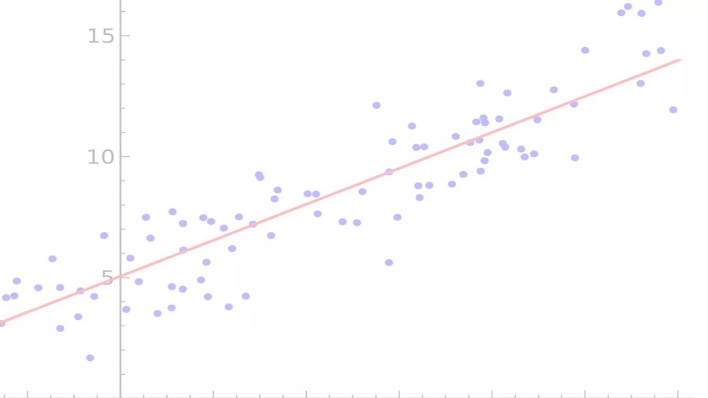
Association Between Maternal Education and Maternal Age in GLM Analysis

In this lecture on Generalized Linear Models in R, the focus is on examining the association between maternal education and maternal age using a dataset on births. The process involves creating a factor variable for maternal education levels, filtering a smaller dataset, visualizing the univariate relationship between maternal education and age, and assessing the normal distribution of maternal age. Simple linear regression is also discussed, demonstrating how to estimate the best-fit line for given data points. Finally, a linear regression model is fitted to investigate the relationship between maternal education and age in the dataset.

• GLM analysis
• Maternal education
• Maternal age
• Linear regression
• Data visualization

sjaz Follow

Uploaded on Oct 04, 2024 | 0 Views

Download Presentation

Please find below an Image/Link to download the presentation.

The content on the website is provided AS IS for your information and personal use only. It may not be sold, licensed, or shared on other websites without obtaining consent from the author. Download presentation by click this link. If you encounter any issues during the download, it is possible that the publisher has removed the file from their server.

Presentation Transcript

1. Generalized Linear Models in R EPID 701, Lecture 12 Tuesday, 18 February 2020 # as you come in, run: library(tidyverse) library(broom) setwd("./..") load("births_cleaned_hw2.rda")

2. Overview Overview Review of Linear Regression Linear Regression in R Review of GLMs Overview of R GLM functions # Homework 4 help!

3. What is the association between maternal What is the association between maternal education and maternal age? education and maternal age? # creating maternal education factor variable: births <- births %>% mutate(meduc = ifelse(meduc==9,NA,meduc), meduc_f = factor(meduc, levels=c(1,2,3,4,5), labels=c("Less Than High School", "High School Graduate or GED", "Some College", "Bachelors Degree", "Masters or PhD"))) # creating a smaller dataset: set.seed(123) births_10k = births %>% filter(complete.cases(.)) %>% as_tibble() %>% sample_n(10000)

4. What is the association between maternal What is the association between maternal education and maternal age? education and maternal age? # univariate relationship births_10k %>% ggplot(aes(x = meduc_f, y = mage)) + geom_jitter(alpha = 0.15)

5. Is maternal age normally distributed? Is maternal age normally distributed? births_10k %>% ggplot(aes(x=mage)) + geom_density()

6. Simple Linear Regression Simple Linear Regression Given data points (x and y), we draw a line of best fit . The slope of the best fit line can be used to summarize the relationship between x and y. We can find the beta estimate and best fit line by minimizing the residual sum of squares : the difference between each observation and it s model- predicted value, squared and summed

7. What is the association between maternal What is the association between maternal education and maternal age? education and maternal age? lm(outcome ~ exposure, data = .) m_linear <- lm(mage ~ meduc, data = births_10k) m_linear > m_linear Call: lm(formula = mage ~ meduc, data = births_10k) For every one-unit increase in maternal education, we would expect an increase of 2.061 years in mean maternal age. Coefficients: (Intercept) meduc 21.780 2.061 https://www.rdocumentation.org/packages/stats/versions/3.6.2/topics/lm

8. Looking at parts of model output Looking at parts of model output # coefficients coef(m_linear) # or m_linear$coefficients > coef(m_linear) # or (Intercept) meduc 21.780088 2.060866 > m_linear$coefficients (Intercept) meduc 21.780088 2.060866 # 95% confidence intervals confint(m_linear) > confint(m_linear) 2.5 % 97.5 % (Intercept) 21.515561 22.04461 meduc 1.973692 2.14804 # AIC value AIC(m_linear) > AIC(m_linear) [1] 61956.14

9. Model summary Model summary > summary(m_linear) summary(m_linear) Call: lm(formula = mage ~ meduc, data = births_10k) Residuals: Min 1Q Median 3Q Max -11.0844 -3.9627 -0.9018 3.0982 27.1590 Coefficients: Estimate Std. Error t value Pr(>|t|) (Intercept) 21.78009 0.13495 161.40 <2e-16 *** meduc 2.06087 0.04447 46.34 <2e-16 *** --- Signif. codes: 0 *** 0.001 ** 0.01 * 0.05 . 0.1 1 Residual standard error: 5.358 on 9998 degrees of freedom Multiple R-squared: 0.1768, F-statistic: 2147 on 1 and 9998 DF, p-value: < 2.2e-16 Adjusted R-squared: 0.1767

10. Model summary Model summary summary(m_linear)

11. broom broom Takes a format that is not in a data frame and converts it to a tidy data frame. Output = a dataframe, no row names! tidy(): summarizes statistical findings augment(): add columns (predictions, residuals, clusters) glance(): one-row summary of model Introduction to broom: https://cran.r-project.org/web/packages/broom/vignettes/broom.html

12. broom broom tidy(m_linear) # A tibble: 2 x 5 term estimate std.error statistic p.value <chr> <dbl> <dbl> <dbl> <dbl> 1 (Intercept) 21.8 0.135 161. 0 2 meduc 2.06 0.0445 46.3 0 glance(m_linear) # A tibble: 1 x 11 r.squared adj.r.squared sigma statistic p.value df logLik AIC BIC deviance df.residual <dbl> <dbl> <dbl> <dbl> <dbl> <int> <dbl> <dbl> <dbl> <dbl> <int> 1 0.177 0.177 5.36 2147. 0 2 -30975. 61956. 61978. 287069. 9998>

13. broom broom augment(): add columns (predictions, residuals, clusters) to a dataset with information from a model augment(m_linear, data = births_10k %>% select(mage, meduc)) %>% head() # A tibble: 6 x 9 mage meduc .fitted .se.fit .resid .hat .sigma .cooksd .std.resid <int> <int> <dbl> <dbl> <dbl> <dbl> <dbl> <dbl> <dbl> 1 24 1 23.8 0.0958 0.159 0.000319 5.36 0.000000141 0.0297 2 32 2 25.9 0.0640 6.10 0.000142 5.36 0.0000923 1.14 3 36 3 28.0 0.0544 8.04 0.000103 5.36 0.000116 1.50 4 27 2 25.9 0.0640 1.10 0.000142 5.36 0.00000299 0.205 5 33 5 32.1 0.112 0.916 0.000438 5.36 0.00000640 0.171 6 24 3 28.0 0.0544 -3.96 0.000103 5.36 0.0000282 -0.740

14. broom broom Or make your own model output summary table! m_linear %>% tidy() %>% bind_cols(m_linear %>% confint_tidy()) # A tibble: 2 x 7 term estimate std.error statistic p.value conf.low conf.high <chr> <dbl> <dbl> <dbl> <dbl> <dbl> <dbl> 1 (Intercept) 21.8 0.135 161. 0 21.5 22.0 2 meduc 2.06 0.0445 46.3 0 1.97 2.15

15. # graphing our model predictions births_10k %>% ggplot(aes(x=meduc_f, y=mage)) + geom_jitter(alpha=0.15) + geom_abline(intercept=21.8, slope=2.06, color="blue", size=2) births_10k %>% ggplot(aes(x=meduc_f, y=mage)) + geom_jitter(alpha=0.15) + geom_smooth(aes(x=meduc, y=mage), method=lm, se=F, color="blue", size=2)

16. Problem 1: Variable distribution Problem 1: Variable distribution But what if the outcome variable is not normal? A binary variable? A categorical variable? An ordinal variable? A count or rate variable? We can address these in R using various outcome distributions. Binomial Multinomial Ordinal Logistic Poisson Quasi-Poisson

17. Problem 2: Non Problem 2: Non- -Independence Independence But what if observations are not independent? Interference between adjacent units? Correlation between outcomes for adjacent units? Shared variables between different observations (clustering)? Repeated measurements of the same units? We can address these problems in R by adding terms to the regression or using more advanced regression / modeling techniques.

18. Solution: Generalized Linear Models Solution: Generalized Linear Models We can solve these problems (and more) by extending our linear model with two new features: 1. An outcome distribution. We can use something other than the normal distribution for our model to show how the variance depends on the mean. 2. A link function. Since we are still using a linear model, we need to transform our data appropriately so that it appears linear ; so that our transformed outcome is linearly related to the exposure and other predictors. In R, we can make these modifications directly in our line of code. We don t have to trick the program to make our models work.

19. glm glm() syntax () syntax You can fit regression models in R using the general-purpose glm() function. The ~ operator separates the outcome from the covariates. glm(outcome ~ exposure + confounder, data=., family=distribution( link )) The model results are usually best saved in an object so that we can easily visualize or manipulate parts of our output. m <- glm(outcome ~ exposure + confounder, data=.)

20. Review of GLMs Review of GLMs Regression model Family Link (g(Y)) Form Y = 0 + 1X1 + kXk linear normal identity R = 0 + 1X1 + kXk linear risk binomial identity ln(R) = 0 + 1X1 + kXk log-risk binomial log logit(R) = 0 + 1X1 + kXk logit-risk binomial logit ln(Y) = 0 + 1X1 + kXk poisson poisson log Y = a continuous dependent variable (outcome) or count variable (poisson models) R = probability for a binomial outcome, e.g., risk (incidence proportion) or prevalence. Family: the distribution of the outcome variable. Link: the functional relation between the dependent variable and the linear combination of covariates EPID716 2019

21. Review of GLMs Review of GLMs Regression model Family Link (g(Y)) Form Y = 0 + 1X1 + kXk linear normal identity R = 0 + 1X1 + kXk linear risk binomial identity ln(R) = 0 + 1X1 + kXk log-risk binomial log logit(R) = 0 + 1X1 + kXk logit-risk binomial logit ln(Y) = 0 + 1X1 + kXk poisson poisson log Y = a continuous dependent variable (outcome) or count variable (poisson models) R = probability for a binomial outcome, e.g., risk (incidence proportion) or prevalence. Family: the distribution of the outcome variable. Link: the functional relation between the dependent variable and the linear combination of covariates EPID716 2019

22. Epidemiology Examples Choose your distribution family link based on what you are estimating: Risk difference Risk ratio family = binomial(link= identity ) family = binomial(link= log ) Rate difference Rate ratio family = poisson(link= identity ) family = poisson(link= log ) Odds ratio family= binomial(link= logit )

23. Review of GLMs Review of GLMs Risk difference: family = binomial(link= identity ) Risk ratio: family = binomial(link= log ) Odds ratio: family= binomial(link= logit ) Rate ratio: family = poisson(link= log ) Rate difference: family = poisson(link= identity ) EPID718 2018

24. Question for the Google Doc Question for the Google Doc What is the association between maternal education and maternal age? Convert your lm() model into a glm() and post your code and estimate in the notes. glm(outcome ~ exposure + confounder, data=., family=distribution( link ))

25. Question for the Google Doc Question for the Google Doc What is the association between maternal education and maternal age? glm_linear <- glm(mage ~ meduc, data = births_10k, family=gaussian(link="identity")) tidy(glm_linear) # A tibble: 2 x 5 term estimate std.error statistic p.value <chr> <dbl> <dbl> <dbl> <dbl> 1 (Intercept) 21.8 0.135 161. 0 2 meduc 2.06 0.0445 46.3 0

26. What is the association between early prenatal What is the association between early prenatal care and preterm birth? care and preterm birth? births_10k %>% group_by(pnc5_f) %>% summarize(n=n(), n_preterm = sum(preterm, na.rm=T), pct_preterm = n_preterm / n * 100) %>% mutate(preterm_RD = pct_preterm - lag(pct_preterm)) # A tibble: 2 x 5 pnc5_f n n_preterm pct_preterm preterm_RD <fct> <int> <dbl> <dbl> <dbl> 1 No Early PNC 851 110 12.9 NA 2 Early PNC 9149 890 9.73 -3.20

27. Linear risk regression Linear risk regression # risk difference glm_rd <- glm(preterm ~ pnc5_f, data = births_10k, family=binomial(link="identity")) The absolute risk of preterm birth among those that received early prenatal care was 3.2 percentage points lower than the absolute risk among those who did not receive early prenatal care. tidy(glm_rd, conf.int = T) # A tibble: 2 x 7 term estimate std.error statistic p.value conf.low conf.high <chr> <dbl> <dbl> <dbl> <dbl> <dbl> <dbl> 1 (Intercept) 0.129 0.0115 11.2 2.60e-29 0.108 0.153 2 pnc5_fEarly PNC -0.0320 0.0119 -2.69 7.25e- 3 -0.0564 -0.00967

28. Log Log- -risk regression risk regression The risk of preterm birth among those that received early prenatal care was 0.75 times the risk among those that did not receive early prenatal care. # risk ratio glm_rr <- glm(preterm ~ pnc5_f, data = births_10k, family=binomial(link="log")) tidy(glm_rr, conf.int = T, exponentiate = T) # or exp(coef(glm_rr)) # A tibble: 2 x 7 term estimate std.error statistic p.value conf.low conf.high <chr> <dbl> <dbl> <dbl> <dbl> <dbl> <dbl> 1 (Intercept) 0.129 0.0890 -23.0 5.16e-117 0.108 0.153 2 pnc5_fEarly PNC 0.753 0.0945 -3.01 2.63e- 3 0.629 0.911

29. Question for the Google Doc Question for the Google Doc What is the association between early prenatal care and preterm birth? Find the odds ratio and post your point estimate and 95% confidence interval in the notes. glm(outcome ~ exposure + confounder, data=., family=distribution( link ))

30. Question for the Google Doc Question for the Google Doc What is the association between early prenatal care and preterm birth? glm_or <- glm(preterm ~ pnc5_f, data = births_10k, family=binomial(link="logit")) tidy(glm_or, conf.int = T, exponentiate = T) # A tibble: 2 x 7 term estimate std.error statistic p.value conf.low conf.high <chr> <dbl> <dbl> <dbl> <dbl> <dbl> <dbl> 1 (Intercept) 0.148 0.102 -18.7 8.92e-78 0.121 0.181 2 pnc5_fEarly PNC 0.726 0.108 -2.96 3.04e- 3 0.590 0.901

31. What about confounding? What about confounding? EPID 716

32. Multivariable regression Multivariable regression glm(outcome ~ exposure + confounder, data=., family=distribution( link )) glm_rd_conf <- glm(preterm ~ pnc5_f + mage + raceeth_f + smoker_f, data = births_10k, family=binomial(link="identity")) # A tibble: 8 x 7 term estimate std.error statistic p.value conf.low conf.high <chr> <dbl> <dbl> <dbl> <dbl> <dbl> <dbl> 1 (Intercept) 8.61e-2 0.0180 4.78 1.73e- 6 5.29e-2 0.121 2 pnc5_fEarly PNC -2.40e-2 0.0117 -2.06 3.94e- 2 -4.80e-2 -0.00225 3 mage 4.66e-4 0.000501 0.930 3.52e- 1 -4.27e-4 0.00137 4 raceeth_fOther 8.59e-3 0.00791 1.09 2.77e- 1 -6.50e-3 0.0246 5 raceeth_fWhite ~ -1.14e-2 0.0164 -0.691 4.89e- 1 -4.00e-2 0.0261 6 raceeth_fAfrica~ 7.73e-2 0.00841 9.19 3.92e-20 6.11e-2 0.0941 7 raceeth_fAmeric~ 7.88e-2 0.0306 2.58 1.00e- 2 2.52e-2 0.144 8 smoker_fSmoker 2.39e-2 0.0102 2.34 1.92e- 2 4.92e-3 0.0445 tidy(glm_rd_conf, conf.int = T)

33. How should we model maternal age? How should we model maternal age? births_10k %>% group_by(mage) %>% summarize(prop_preterm = mean(preterm, na.rm=T)) %>% ggplot(aes(x=mage, y=prop_preterm)) + geom_col() 33

34. Functional form Functional form - - linear linear ff_mage <- glm(preterm ~ mage, data = births_10k, family=binomial(link="identity")) tidy(ff_mage, conf.int = T) # linear # A tibble: 2 x 7 term estimate std.error statistic p.value conf.low conf.high <chr> <dbl> <dbl> <dbl> <dbl> <dbl> <dbl> 1 (Intercept) 0.115 0.0143 8.03 9.99e-16 0.0895 0.141 2 mage -0.000545 0.000506 -1.08 2.81e- 1 -0.00144 0.000361

35. Functional form Functional form - - linear linear # creating dataframe with predictions m.pred <- as_tibble(predict(ff_mage, type = "response", se.fit = T)) m.pred$lower <- m.pred$fit - (1.96*m.pred$se.fit) # lower bounds m.pred$upper <- m.pred$fit + (1.96*m.pred$se.fit) # upper bounds m.pred$x <- births_10k$mage # actual age values m.pred$y <- births_10k$preterm # actual mortality values m.pred

36. Functional form Functional form - - linear linear # creating dataframe with predictions # A tibble: 10,000 x 7 fit se.fit residual.scale lower upper x y <dbl> <dbl> <dbl> <dbl> <dbl> <int> <dbl> 1 0.102 0.00353 1 0.0950 0.109 24 0 2 0.0976 0.00371 1 0.0903 0.105 32 1 3 0.0954 0.00516 1 0.0853 0.106 36 1 4 0.100 0.00302 1 0.0944 0.106 27 0 5 0.0970 0.00403 1 0.0891 0.105 33 0 6 0.102 0.00353 1 0.0950 0.109 24 0 7 0.101 0.00312 1 0.0947 0.107 26 0 8 0.0981 0.00343 1 0.0914 0.105 31 0 9 0.0965 0.00438 1 0.0879 0.105 34 0 10 0.0992 0.00307 1 0.0932 0.105 29 0 # ... with 9,990 more rows m.pred <- as_tibble(predict(ff_mage2, type = "response", se.fit = T)) m.pred$lower <- m.pred$fit - (1.96*m.pred$se.fit) # lower bounds m.pred$upper <- m.pred$fit + (1.96*m.pred$se.fit) # upper bounds m.pred$x <- births_10k$mage # actual age values m.pred$y <- births_10k$preterm # actual mortality values m.pred

37. Functional form Functional form - - linear linear ggplot(m.pred) + geom_point(aes(x=x, y=fit)) + # predictions geom_ribbon(aes(x=x, ymin=lower, ymax=upper, alpha=0.01), fill="#d1e5f0", show.legend = F) + # 95% CI geom_smooth(aes(x=x, y=y), color = "blue", method = "loess", se = F, show.legend = F) + # actual labs(title="Linear Model", x="Maternal Age", y="Estimated Risk (95% CI) of Preterm Birth", subtitle="Blue solid line is loess, dots are model predictions with confidence interval bands.") + theme_bw()

38. Bad fit :( Functional form Functional form - - linear linear ggplot(m.pred) + geom_point(aes(x=x, y=fit)) + # predictions geom_ribbon(aes(x=x, ymin=lower, ymax=upper, alpha=0.01), fill="#d1e5f0", show.legend = F) + # 95% CI geom_smooth(aes(x=x, y=y), color = "blue", method = "loess", se = F, show.legend = F) + # actual labs(title="Linear Model", x="Maternal Age", y="Estimated Risk (95% CI) of Preterm Birth", subtitle="Blue solid line is loess, dots are model predictions with confidence interval bands.") + theme_bw()

39. Other functional forms Other functional forms Quadratic: poly(mage,2) Polynomial: poly(mage,3) Splines: rcs(mage,c(20,25,30)) Interaction terms: mage*pnc5_f Indicator terms and categorical: catg(mage) https://r4ds.had.co.nz/model-basics.html#formulas-and-model-families

40. Question for the Google Doc Question for the Google Doc Graph the functional form of maternal age as a quadratic variable and post your plot to the google doc! Name your quadratic model ff_mage2

41. Question for the Google Doc Question for the Google Doc

42. Model testing Model testing > AIC(ff_mage); logLik(ff_mage) [1] 6504.265 'log Lik.' -3250.132 (df=2) AIC(ff_mage); logLik(ff_mage) AIC(ff_mage2); logLik(ff_mage2) > AIC(ff_mage2); logLik(ff_mage2) [1] 6469.218 'log Lik.' -3231.609 (df=3) > anova(ff_mage, ff_mage2, test="LRT") Analysis of Deviance Table Model 1: preterm ~ mage Model 2: preterm ~ poly(mage, 2) Resid. Df Resid. Dev Df Deviance Pr(>Chi) 1 9998 6500.3 2 9997 6463.2 1 37.047 1.153e-09 *** --- Signif. codes: 0 *** 0.001 ** 0.01 * 0.05 . 0.1 1 anova(ff_mage, ff_mage2, test="LRT")

43. Next Steps Next Steps Lecture on 2/20: Effect measure modification using glms More data visualization with ggplot2