Understanding the Value of Money and Standards
The value of money refers to its purchasing power, which is influenced by the price level of goods and services. Different standards, such as wholesale, retail, and labor, help measure the value of money. Money can have internal and external value, affecting domestic and foreign transactions. The Quantity Theory of Money explains how the value of money changes over time based on the quantity of money in circulation.
Download Presentation

Please find below an Image/Link to download the presentation.
The content on the website is provided AS IS for your information and personal use only. It may not be sold, licensed, or shared on other websites without obtaining consent from the author. Download presentation by click this link. If you encounter any issues during the download, it is possible that the publisher has removed the file from their server.
E N D
Presentation Transcript
Value of Money: The term value of money means the purchasing power of money. It refers to the quantity of goods and services that can be bought by a unit of money. According to D. H. Robertson, The value of money means the amount of things in general which will be given in exchange for a unit of money Value of Money- A relative concept: The value of money is a relative concept. The value of money or purchasing power of money depends upon the price level of goods and services to be purchased with money. Thus, the value of money is inversely related to the price level. The money buys more when prices of goods and services are low and money buys less when prices are high.
Standards of value of money: 1. Wholesale Standard: According to this standard, the value of money is expressed in terms of prices of all those commodities whish are traded in the wholesale market. It includes raw materials, semi-finished and finished goods which are traded in large quantities 2. Retail standard: According to this standard, the value of money express in terms of those goods and services which are purchased by average family for consumption purpose. There are purchased in small quantities. 3. Labour Standard: According to this, the value of money is calculated from the average wage rate payable to the labour for a day s work.
Types of value of money: Value of money is of two types: 1. Internal value of money: It refers to the purchasing power of money within a country. It is value of national currency over domestic goods and services. It is based on the internal price level. 2. External Value of money: It refers to the value of money over foreign goods and services. It is the purchasing power of the national currency outside the currency. It is based on the exchange rate between two currencies.
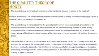
The Quantity Theory of money: This theory try to explain the determination of the value of money and variations in its value over a period of time. This theory was made by writers like Locke and David Hume in 18thcentury, Irving Fisher, Alfred Marshall, A.C. Pigou and Friedman in the 20thcentury. It states that, other things remaining the same, the general price level varies directly and proportionately with the quantity of money. Generally the value of money or the price level does not remain constant but fluctuates often. When the price level rises, the value of money declines and when the price level declines, the value of money rises. There are two approaches to the traditional quantity theory of money, 1. The American version or cash transaction version, and 2. The Cambridge version or cash balance version.
Fishers Quantity Theory of Money or Cash Transaction Approach. The Cash transaction approach of the quantity theory of money was provided by the American economist Irving Fisher in his book- The Purchasing Power of Money (1911). According to Fisher, Other things remaining unchanged, as the quantity of money in circulation increases, the price level also increases in direct proportion and the value of money decreases and vice versa . Fisher s quantity theory is explained with the help of his famous equation of exchange: MV = PT or P = MV/T Where, M the total quantity of money of all types. V is the velocity of circulation of money. The product MV is the total supply of money in a year. T is the total amount of goods and services exchanged for money. p is the price per unit, Hence the product PT is the total value of all the transactions for which money is used.
Like other commodities, the value of money or the price level is also determined by the demand and supply of money. 1. Supply of Money: The supply of money consists of the quantity of money in existence (M) multiplied by the velocity of money (V). In Fisher s equation, V is the velocity of money which means the average number of times a unit of money turns over or changes hands. Thus, MV refers to the total volume of money in circulation during a period of time. ii. Demand for Money: Money is demanded for transaction purposes. The demand for money is equal to the total market value of all goods and services transacted. It is obtained by multiplying total amount of things (T) by average price level (P). MV=PT suggest that in an economy, the total value of all goods sold during any period PT, is equal to the total quantity of money MV spent during that period. The equation further denotes that the price level is directly related to MV and inversely related T.
Fisher quantity theory of money is explained with the help of diagram. P=f(M) y y ?4 1/P Price level Value of money (A) (B) 1/?2 ?2 1/?4 1/P=f(M) P x O M ?2 Money supply ?4 x M O ?2 ?4 Money supply
The diagram A shows the effect of change in quantity of money on the price level. When the quantity of money is M, price level is P. When the quantity of money doubled to M2, the price level is also raised to P2. This relationship is expressed by the curve P=f(M). The diagram B shows the inverse relationship between the quantity of money and value of money. When the quantity of money is M1, the value of money is 1/P. When the quantity of money increased by M4, the value of money is reduced to 1/P4. This inverse relationship between quantity of money and the value of money is expressed by the curve 1/P=f(M).
Assumptions of Fishers Quantity Theory: 1. Constant Velocity of Money: According to Fisher, the velocity of money (V) is constant and is not influenced by the changes in the quantity of money. 2. Constant Volume of Trade or Transactions: Total volume of trade or transactions (T) is also assumed to be constant and is not affected by changes in the quantity of money. 3. Price Level is a Passive Factor: According to Fisher the price level (P) is a passive factor which means that the price level is affected by other factors of equation, but it does not affect them
4. Money is a Medium of Exchange: The quantity theory of money assumed money only as a medium of exchange. Money facilitates the transactions. 5. Constant Relation between M and M : Fisher assumes a proportional relationship between currency money (M) and bank money (M ). 6. Long Period: The theory is based on the assumption of long period. Over a long period of time, V and T are considered constant.
Criticisms of Quantity Theory of Money: 1. Unrealistic Assumption: The assumption that P is passive, V and T are constant, is highly unrealistic. P is not passive, it affect the other elements in the equation. Similarly V is not independent, it changes with a change in M 2. Unrealistic Assumption of Long Period: The quantity theory of money has been criticized on the ground that, it provides a long-term analysis of value of money. It throws no light on the short-run problems. Keynes has aptly remarked that in the long-run we are all dead . Actual problems are short-run problems. 3. Unrealistic Assumption of full Employment: Keynes fundamental criticism of the quantity theory of money was based upon its unrealistic assumption of full employment. Full employment is a rare phenomenon in the actual world. 4. Static Theory: The quantity theory assumes that the values of V, V , M and T remain constant. But, in reality, these variables do not remain constant. Hence, this theory is static nature.
5. Simple Truism: The equation of exchange (MV = PT) is a mere truism and proves nothing. The equation does not tell anything about the causal relationship between money and prices; it does not indicate which is the cause is and which is the effect. 7. Fails to Explain Trade Cycles: The quantity theory does not explain the cyclical fluctuations in prices. It does not tell why during depression the prices fall even with the increase in the quantity of money and during the boom period the prices continue to rise at a faster rate in spite of the adoption of tight money and credit policy. 8. One-Sided Theory: Fisher s transactions approach is one- sided. It takes into consideration only the supply of money and its effects and assumes the demand for money to be constant. ****** ******* *************
The Cash-balance Approach or Cambridge equation of exchange: The Cash balance approach was provided by some of the economists of the Cambridge University such as Alfred Marshall, A C Pigou, D H Robertson and J M Keynes. The equation is based on the store of value function of money and cash balance held by the people to make day to day expenditures. According to the Cambridge economists, the value of money is determinised in terms of supply and demand. Features: According to this approach, the price level depends upon the demand for and supply of money. Hence, the changes in the value of money are caused by either change in the demand for or supply of money. According to the theory, the supply of money is a stock rather than a flow. It comprises of all the cash and bank deposits. The demand for money implies a demand for cash balance. Cash balance is that proportion of the real income which the people to hold in the form of money. 4. Given the supply of money at a point of time, the value of money is determined by the demand for cash balances. 1. 2. 3.
1. Marshalls Equation: According to Marshall, The demand for money as a stable function of money, income and property. Marshall s equation is as follows: M = KPY Where, M Total supply of money (currency cash and demand deposits) K is the fraction of money income held in cash. Y is the aggregate real national income. P is the price level. ? ?? or Value of money 1 ?=?? Thus, the price level is P= ? According to Marshall P that is the value of money can be found by dividing KY, that is the quantity of goods which the community demands at a particular point of time, by M that is total supply of money at a particular point of time.
According to Pigou, the demand for money consists not only of legal tender money, but also bank deposits. Hence, the equation has modified as. ?? P= ? [?+ 1 ? ] Where: C= denotes the ready cash with the public (1-c)= represents the amount of ready cash kept in the form of bank deposits h =is the percentage of cash reserves against bank deposits held by the bank. So, [? + 1 ? ] represents the total amount of cash in the community at any particular time. According to Pigou, the purchasing power of money is influenced by both supply of money (M) and the demand for money (K). He considers K as more significant than M in influencing the changes in the value of money.
According to Pigou, the demand curve for money has a uniform unitary elasticity. This is shown in the diagram as follows. Y D ?1 ?2 ?3 Value of money ?1 ?2 ?3 ?1 X O M1 ?2 ?3 Money demanded and supplied
In the above diagram, D?1 is the demand curve for money and Q1M1, Q2M2 and Q3M3 are the supply curves of money drawn on the assumption that the supply of money is fixed at a point time. When the supply of money increases from OM1 to OM2, the value of money is reduced from OP1 to OP2. If the supply of money increases from OM1 to OM3, the value of money is reduced by exactly from OP1 to OP3. Thus, It shows changes in the value of money exactly in the reverse proportions to the supply of money.
Robertsons Equation: To determine the value of money, Robertson formulated an equation similar to that of Pigou. ? ?? M = PKT or P= Where, M = is the total quantity of money. T = is the total volume of goods and services purchased during a year. K= is the fraction of T which people wish to hold in the form of cash. Thus the equation points out that P changes directly with M and inversely with K or T. Keynes Equation: Keynes gave his Real balance quantity equation as an improvement over other cash balance equations. According to him, people always want to have some purchasing power to finance their day to day transactions.
The amount of purchasing power depends partly on their taste and habits and partly on their wealth. This demand for money is measured by consumption units. N= PK +R?1 Where, N represents quantity of money in circulation. P the price level of consumption goods. K is the amount of the consumption goods which the people desire to hold. ?1 - is the amount of the consumption goods which the people hold in the form of bank deposits. R is the cash reserve ratio of the banks. In the above equation, if K is constant, a proportionate increase in N (amount of money) will lead to a proportionate increase in price level ( P ) According to Keynes, in the short period, K ?1 and remain constant. So a change in N will cause a direct proportionate change in P. In the long run K ?1 and R may not remain constant. So a change in N may influence K,?1and R.
Criticisms: 1. Simple Truism: The Marshall equation establishes proportionate relationship between the quantity of money and the price level M=KPM, assuming all other factors to be constant. It does not tell anything new. 2. Role of rate of interest ignored: The cash balance theory excludes the role of rate of interest in explaining the changes in the price level which is very important in determining the demand for money. 3. Ignored the speculative motive: This approach has not properly analysed various motives for holding money. It ignored the speculative motive for holding money which causes changes in the demand for money. 4. K and T assumed constant: Fisher also assume that K and T remain constant. This is possible in a static situation
But in dynamic conditions. So the theory is inadequate to explain the dynamic price behavior in the economy. 5. The cash balance approach is narrow: This approach fail to explain purchasing power of money in terms of capital goods. But it considered only consumption goods. 6. Neglects other factors: This theory is narrow because K is also determined by factors other than real income, such as, the price level, the monetary and business habits and political conditions in the country. 7. Unitary elasticity of demand: The Cambridge equation assumes that the elasticity demand for money is unity. This is unrealistic assumption because the elasticity of demand cannot be unity in the modern day in the progressive and dynamic society.
Friedmans Restatement of Quantity Theory: Milton Friedman in his essay, the quantity theory of money a restatement published in 1956 and restated the old quantity theory of money. According to Friedman, quantity theory is a theory of demand for money and not a theory of output, income or prices. Secondly, Friedman distinguishes between two types of demand for money. In the first type, money is demanded for transaction purposes. It serves as a medium of exchange. But in the second type, money is demanded because it is considered as an asset or capital goods. The demand for money depends on three factors: (a) The total wealth to be held in various forms of assets. (b) The price or return from these various assets and (c) Tastes and preferences of the asset holders.
Friedman considers five different forms in which wealth can be held, namely, money (M), bonds (B), equities (E), physical non-human goods (G) and human capital (H). In a broad sense, total wealth consists of all types of income . Each form of wealth has a unique characteristic of its own and a different yield. 1. Money is the broadest sense, it includes currency, demand deposits and time deposits which yield interest on deposits. 2. Bonds are defined as claim to a time stream of payments that are fixed in nominal units. 3. Equities are defined as a claim to a time stream of payments that are fixed in real units. 4 Physical goods or non-human goods are inventories of producer and consumer durable. 5. Human capital is the productive capacity of human beings
Five forms of wealth constitutes the current value of wealth which can be expressed as: W = y/r Where W - the current value of total wealth, Y -is the total flow of expected income from the five forms of wealth, r - is the interest rate. This equation shows that wealth is capitalized income.
By combining all the factors, the demand function for money may be given as M/P = f (y, w; Rm, Rb, Re, gp, u) Where M is the total stock of money demanded; P is the price level; is the real income; w is the fraction of wealth in non-human form: Rm is the expected nominal rate of return on money; Rb is the expected rate of return on bonds, including expected changes in their prices. Re is the expected nominal rate of return on equities, including expected changes in their prices; gp=(1/P) (dP/dt) is the expected rate of change of prices of goods and hence the expected nominal rate of return on physical assets; u = stands for variables other than income that may affect the utility attached to the services of money.
Thus, according to Friedman, a change in the stock of money brings about changes in the same direction in the price level or income or both. So long as the demand for money remains stable, a change in its supply will bring about change in the price level.
Friedman's quantity theory of money can be explained with help of following diagram. clip_image004
The income (Y) is measured on the vertical axis and the demand for and the supply of money are measured on the horizontal axis. MD is the demand for money curve which varies with income. MS is the money supply curve which is perfectly inelastic to changes in income. The two curves intersect at E and determine the equilibrium income OY. If the money supply rises, the MS curve shifts to the right to M1S1. As a result, the money supply is greater than the demand for money which raises total expenditure until new equilibrium is established at E1 between MD and M1S1, curves. The income rises to OY1. Thus, Friedman presents the quantity theory as the demand for money is assumed to depend on asset prices or relative returns and wealth or income. He observed that the demand function for money is stable and hence any change in the supply of money will affects the level of economic activity.
Criticisms: 1. Very Broad Definition of Money: Friedman has been criticized for using the broad definition of money which not only includes currency and demand deposits ( 1) but also time deposits with commercial banks (M2). 2. Money not a Luxury Good: Friedman regards money as a luxury good because of the inclusion of time deposits in money. But no such luxury effect has been found in many other economies. 3. More Importance to Wealth Variables: In Friedman s demand for money function, wealth variables are preferable to income and the operation of wealth and income variables simultaneously does not seem to be justified. As pointed out by Johnson, income is the return on wealth, and wealth is the present value of income.
4. Money Supply not Exogenous: Friedman takes the supply of money to be unstable. The supply of money is varied by the monetary authorities in an exogenous manner in Friedman s system. But it is endogenous. 5. Ignores the Effect of Other Variables on Money Supply: Friedman also ignores the effect of prices, output or interest rates on the money supply. But there is considerable empirical evidence that the money supply can be expressed as a function of the above variables. 6. Does not consider Time Factor: Friedman does not tell about the timing and speed of adjustment or the length of time to which his theory applies. 7. No Positive Correlation between Money Supply and Money GNP: Money supply and money GNP have been found to be positively correlated in Friedman s findings. But, according to Kaldor, in Britain the best correlation is to be found between the quarterly variations in the amount of cash held in the form of notes and coins by the public and corresponding variations in personal consumption at market prices, and not between money supply and the GNP.
Index Numbers: An index number is a statistical device to measure the changes in the value of money over a period of time. It can be defined as statistical measure with a purpose of showing average changes in one or more related variables between two periods of time ( 2015 and 2020 ) or two places or countries. According to Spiegel, An index number is a statistical measure designed to show changes in a variable or a group of related variables with respect to time, geographical location or other characteristics. According to Croxton and Cowdon: Index number are devices for measuring differences in the magnitude of a phenomenon are measured from time to time or from place to place.
Types Of Index numbers: 1. Price Index number: Price index number is an index number which compares the prices for group of commodities at a certain period or at a location with prices of base period. Price index is used to measure the value of money. Price index may be i. Wholesale Price Index Number: Wholesale price index number are constructed on basis of the wholesale price of certain selected commodities. These commodities are traded in wholesale markets. The commodities included are raw-materials, foodstuffs, semi-finished goods and manufacturers. ii. Retail Price Index Number: Retail Prices Index Number are constructed on basis of retail prices of final consumption goods. These commodities are traded in retail market. These index number will measure the purchasing power of money to the final consumer. iii. Cost of Living Index Number: This index number takes into account the prices of important commodities which are consumed by common people. The different prices used are retail prices. This index number may be constructed to measure changes in the cost of living of the different sections of society like working class, different income groups, etc.
2. Quantity Index Number: It studies the changes in the volume of goods produced or consumed. They are useful to study the changes in output in different sectors of the economy. It includes, a. Agricultural Index Number: They are constructed to measure changes in the production of agricultural commodities between different points of time. They are used for agricultural planning and cost price regulations, etc. b. Industrial Index Number: It refers to the index numbers measuring changes in the value of industrial production at different points of time. c. International Index Number: These index number measures the changes in the prices of goods traded among the different countries. These can be prepared separately for imports and exports. d. Trade Index Number: d. These are helpful in measuring the relative changes in the trade and commercial activities.
e. Investment index number This index number are used to measure the trends in the level of investment of the country. It also used to measure the trends in the prices of securities in the financial market. 3. Value Index Number: These index number compare the total value of a certain period with the total value of the base period. In this index number both prices and quantities are taken into consideration.
Steps followed in the construction of price index numbers: The purpose of Index Number: The purpose for which the index numbers are to be constructed must be clearly defined. Since there are many types of index numbers, every index number is of limited and particular use. Decisions regarding choice of commodities, selection of base period, collection data etc, very much depends upon the purpose of an index number. 1. 2. Selection of Base period: Base year is a year in the past with which current period price level is to be compared. The base may be a year, a month or even a day. While selecting base year two conditions should be taken into account. They are, a. Base year should be a normal year. Abnormal events like flood, drought, earthquake etc should not taken place in the base year.
b. A base year should not be a very distant in the past because the things which are available in the base year may not be available in the current year. 3. Selection of commodities: Commodities to be selected depend upon the purpose or objectives of the index number. In selecting the different commodities, the given points are to be taken into consideration. a. The item must represent the consumption habit of the group of people concerned. b. The items selected must be representative and they should be neither too many nor too few. c. The commodity selected should be off standard quality. 4. Collection of Data. The reliability of the index number depends upon the accuracy of the data used for its construction. Prices may be collected either from the published records or from primary sources. Similarly prices may be collected either from wholesale market or from the retail market.
Generally, wholesale prices are used in the construction of general price index number and retail prices are used in the construction of cost of living index number. 5. Selection of Weights: Weights are assigned to different commodities to express their relative importance in the pattern of consumption. Weights may be given in terms of value or quantity. In simple index number equal importance is given to all the items collected. But this index number does not give us a correct picture regarding the changes in economic activity. 6. Choice of Average: The construction of general price index number involves a process of combining several prices in such a way that a single number may reflect the overall changes. The two methods of averages that are commonly used are the arithmetic mean and the geometric mean.
Uses of Index Numbers: 1. Used to Measure Cost of Living: Index numbers are used to know the changes in the cost of living. The cost of living index is the basis for adjusting wages and other allowances and also of wage negotiations and wage contracts. 2. Economic Barometer: Index numbers are used to measure the relative changes in various economic phenomena like level of prices, production, employment, trade, agriculture, industry, foreign trade, etc. Thus, they give a better idea of changes in various economic variables. 3. Used in Measuring the Value of money. Index number helps to measure the purchasing power of money. This enables the government to take appropriate measure to stabilise the purchasing power of money.
4. Used in Economic Policies: Index numbers measure the changes in the economic variables and with this information help the planners to formulate appropriate economic policies. 5. Helps in international comparison: Index number are used to make comparison among different countries. It is with the help of various types of index numbers, the growth and growth rate of different countries is compared and analysed. 6. Indicators of the economic progress: Production index is goods indicators of the economic progress taking place in the different sectors of the economy. They can also be used to forecast future trends in production. Such index number are extremely useful for planning.
7. To compare the standard of living: Index number may measure the cost of living of different classes of people and also of different regions. This helps in comparing the standard of living of different people. 8. In Determining the foreign exchange rate: Index number of wholesale price of two countries are used to determine their rate of foreign exchange. They are the basis of the purchasing power parity theory which determines the exchange rate between two countries. -------- ----------- --------
Inflation: Inflation is a situation in which there is rise in the general price level and fall in the value of money. In other words, it refers to a situation of continuous rise in the general price level over a period of time. According to Coulbourn, inflation is too much money chasing too few goods According to J M Keynes, inflation is the result of the excess of aggregate demand over the available aggregate supply and true inflation starts only after full employment. Features of Inflation: 1. It is a process of persistent rise in prices. 2. It is a monetary phenomenon & is generally caused by excessive money supply. 3. It is caused by excess of demand over the supply of everything. 4. It starts only after full employment.
Classification of Inflation: 1. On the basis of rate of Increase in Prices: a. Creeping Inflation: It refers to a situation where there is a very mild rise in prices. The price level is about 1 3% annum. This kind of inflation is generally considered to be beneficial to the economy as it favours trade, industry, investment and growth. b. Walking Inflation: It is a situation where the rise in price is about 3-6% per annum. It is faster than creeping inflation. C. Running Inflation: It is a situation where the price level rises very fast. In this case price level doubles every 3 years, the sustained rise in prices is about 10 %. d. Galloping Inflation: It refers to a situation where the price level rises very rapidly. In this case, the price level doubles up every 10 months, some times every week.
2. On the basis of governments Reaction: a. Open Inflation: It is an inflationary situation in which prices are permitted to rise without being suppressed by price controls or other similar techniques by the govt. b. Suppressed and Repressed Inflation: It is a situation under which prices are prevented from rising high through price controls and rationing by the govt. 3. On the basis of employment: a. Partial Inflation: Rise in the prices before full employment is reached is called semi inflation or partial inflation. b. True Inflation: Rise in prices after full employment is reached is called true or pure inflation.
4. On the basis of number of goods covered: a. Comprehensive Inflation: It refers to a situation where the prices of all goods rise throughout the economy. it is also called as economy-wide inflation. b. Sporadic Inflation: It refers to a situation where the prices of only some goods rise. For an example of this type of inflation is a rise in the prices of food grains caused by food shortages resulting from crop failures that are sporadic inflation. 5. On the basis of time: a. Wartime inflation: It is a inflation caused by excessive expenditure on war. b. Post war inflation: It takes place immediately after the war time when the demand increases. c. Peace Time Inflation: It occurs during peacetime due to excess government expenditure over its revenue.
6. On the basis of inducement: a. Deficit induced inflation: Inflation caused by deficit financing undertaken by the government is called deficit. b. Wage induced inflation: Inflation caused by a rise in wage unmatched by a rise in productivity of power is called wage induced inflation. c. Profit induced inflation: It is caused by too high profit earned by the producers is called profit induced inflation. 7. On the basis of factors responsible for inflation: a. Demand-pull Inflation: Inflation arising out of excess demand for goods as against the supply of goods at the full employment level leads to demand pull inflation.
b. Cost-push inflation: When a rise in the cost of production caused by the higher wages leads to rise in prices in goods. This situation is caused cost-push inflation. ------- ---------- ----------


