Understanding Correlation in Research Designs
Correlation
CHAPTER 15
A research design reminder
Experimental designs
◦
You directly manipulated the independent variable
Quasi-experimental designs
◦
You examined naturally occurring groups
Correlational designs
◦
You just observed the independent variable
Defining Correlation
Co-variation or co-relation between two variables
These variables change together
Usually scale (interval or ratio) variables
Correlation does NOT mean causation!
Correlation versus Correlation
Correlational designs = research that doesn’t manipulate
things because you can’t ethically or don’t want to
◦
You can use all kinds of statistics on these depending on what
you types of variables you have
Correlation can be used in any design type with two
continuous variables
Correlation Coefficient
A statistic that quantifies a relation between two variables
Tells you two pieces of information:
◦
Direction
◦
Magnitude
Correlation Coefficient
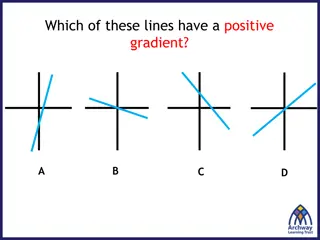
Direction
◦
Can be either positive or negative
◦
Positive: as one variable goes up, the other variable goes up
◦
Negative: as one variable goes up, the other variable goes
down
Positive Correlation
Association between variables such that high scores on one
variable tend to have high scores on the other variable
◦
A direct relation between the variables
Negative Correlation
Association between variables such that high scores on one
variable tend to have low scores on the other variable
◦
An inverse relation between the variables
A Perfect Positive Correlation
A Perfect Negative Correlation
Correlation Coefficient
Magnitude
◦
Falls between -1.00 and 1.00
◦
The value of the number (not the sign) indicates the strength
of the relation
A visual guide
Check Your Learning
Which is stronger?
◦
A correlation of 0.25 or -0.74?
Misleading Correlations
Something to think about
◦
There is a 0.91 correlation between ice cream consumption
and drowning deaths.
◦
Does eating ice cream cause drowning?
◦
Does grief cause us to eat more ice cream?
Another silly example
Correlation Overall
Tells us that two variables are related
◦
How they are related (positive, negative)
◦
Strength of relationship (closer to | 1 | is stronger; farther
away from 0)
Lots of things can be correlated – must think about what
that means
Limitations of Correlation
Correlation is not causation
◦
Invisible third variables
Three Possible Causal Explanations for a Correlation:
Causation Direction
Restricted Range
◦
A sample of boys and girls who performed in the top 2% to 3% on
standardized tests - a much smaller range than the full population
from which the researchers could have drawn their sample
Limitations of Correlation
Restricted Range Cont.
If we only look at the older students between the ages of 22
and 25, the strength of this correlation is now far smaller,
just 0.05
Limitations of Correlation
The effect of an outlier
◦
One individual who both studies and uses her cell phone more
than any other individual in the sample changed the
correlation from 0.14, a negative correlation, to 0.39, a much
stronger and positive correlation!
The Pearson Correlation
Coefficient
A statistic that quantifies a linear relation between two
scale variables
Symbolized by the italic letter
r
when it is a statistic based
on sample data
Symbolized by italicized
ρ
(rho) when it is a population
parameter
Correlation Hypothesis Testing
Step 1. Identify the population, distribution, and
assumptions
Step 2. State the null and research hypotheses
Step 3. Determine the characteristics of the comparison
distribution
Step 4. Determine the critical values
Step 5. Calculate the test statistic
Step 6. Make a decision
Assumptions - Step 1
Random selection?
X and Y at least scale variables?
Linear relationship between variables? (linearity)
Outliers?
Homoscedasticity? (for real this time!)
◦
Each variable must vary approximately the same at each point
of the other variable
◦
See scatterplot for UFOs, megaphones, snakes eating dinner.
X and Y are both normal? (normality)
Assumptions - Step 1
(linearity)
Open the data in JASP and make sure the variables are
correct
Descriptives
Descriptive Statistics
Move both variables
over to the “Variables” box
Plots
Correlation Plot
Look at top right graph
Close to a line? Linear!
Assumptions - Step 1 (outliers)
Look at the graph in the same graph as linearity
If data points are way off, consider them outliers see
examples over here
Our graph:
We don’t have anything that looks like that, so we’re good!
Assumptions - Step 1
(normality)
T-test
One Sample T-Test
Under “Assumptions” select
“Normality”
Remember, here we want p > .05
Made it!
Assumptions – Step 1
(homoscedasticity)
How to assess homoscedasticity?
◦
Look at our scatterplot from earlier
◦
Outlier the group of dots
◦
To meet homoscedasticity, needs to the box-like (i.e. the
spread across one axis should remain about the same as you
move across the other axis)
◦
Ours looks pretty box-like,
so we’re good!
Assumptions – Step 1
(homoscedasticity) cont.
Examples of not meeting homoscedasticity:
◦
If you don’t meet homoscedasticity your data is considered
heteroscedastic
Step 2- Sate your hypotheses
Null Hypothesis: no correlation between variable 1 and
variable 2
Research Hypothesis: correlation between variable 1 and
variable 2
For our example:
◦
Null:
r
for cholesterol and TV time = 0
◦
No correlation between cholesterol and TV time
◦
Research:
r
for cholesterol and TV time ≠ 0
◦
Correlation between cholesterol and TV time
Step 3- Find
r
and
df
df
=
N
– 2
To get
r
we will used JASP
◦
“Regression”
“Correlation Matrix”
move your variables
over
◦
Make sure “Pearson’s” is selected
select “Display pairwise
table”
◦
Select “Confidence intervals” if needed
Step 4
Find the
t
critical
value
◦
Use the
df
and
p
critical to determine
t
critical
using the two-
tailed section of the
t
distribution table
Step 5
Calculate the
t
actual
given your
r
value
http://vassarstats.net/tabs_r.html
Step 6
If you reject the null:
◦
There is a significant correlation (relationship)
If you fail to reject the null:
◦
There was not a significant correlation (relationship) between
the variables in the dataset
Effect Size?
r
is often considered an effect size
◦
Most people square it though to
r
2
, which is the same as
ANOVA effect size
◦
You can also switch
r
to Cohen’s
d
, but people are moving away
from doing this because
d
normally is reserved for nominal
variables
Confidence Intervals
Involves Fisher’s
r
to
z
transformation and is generally pretty
yucky
◦
Which means people do not do them unless they are required
to
Correlation and Psychometrics
Psychometrics is used in the development of tests and
measures
Psychometricians use correlation to examine two important
aspects of the development of measures—reliability and
validity
Reliability
A reliable measure is one that is consistent
Example types of reliability:
◦
Test-retest reliability
◦
Split-half reliability
Cronbach’s alpha (aka coefficient alpha)
◦
Want to be bigger than .80
Validity
A valid measure is one that measures what it was designed
or intended to measure
Correlation is used to calculate validity, often by correlating
a new measure with existing measures known to assess the
variable of interest
Validity
Correlation can also be used to establish the validity of a
personality test
Establishing validity is usually much more difficult than
establishing reliability
Buzzfeed!
Partial Correlation
A technique that quantifies the degree of association
between two variables after statistically removing the
association of a third variable with both of those two
variables
Allows us to quantify the relation between two variables,
controlling for the correlation of each of these variables
with a third related variable
Partial Correlation
We can assess the correlation between number of absences
and exam grade, over and above the correlation of
percentage of completed homework assignments with
these variables
Research designs like experimental, quasi-experimental, and correlational serve different purposes in studying variable relationships. Correlation does not imply causation and can be positive or negative, indicating how two variables change together. The correlation coefficient quantifies this relationship, providing information on direction and magnitude, leading to different types of correlations like positive and negative correlations, as well as perfect correlations.

Download Presentation

Please find below an Image/Link to download the presentation.
The content on the website is provided AS IS for your information and personal use only. It may not be sold, licensed, or shared on other websites without obtaining consent from the author. Download presentation by click this link. If you encounter any issues during the download, it is possible that the publisher has removed the file from their server.
E N D
Presentation Transcript
Correlation CHAPTER 15
A research design reminder Experimental designs You directly manipulated the independent variable Quasi-experimental designs You examined naturally occurring groups Correlational designs You just observed the independent variable
Defining Correlation Co-variation or co-relation between two variables These variables change together Usually scale (interval or ratio) variables Correlation does NOT mean causation!
Correlation versus Correlation Correlational designs = research that doesn t manipulate things because you can t ethically or don t want to You can use all kinds of statistics on these depending on what you types of variables you have Correlation can be used in any design type with two continuous variables
Correlation Coefficient A statistic that quantifies a relation between two variables Tells you two pieces of information: Direction Magnitude
Correlation Coefficient Direction Can be either positive or negative Positive: as one variable goes up, the other variable goes up Negative: as one variable goes up, the other variable goes down
Positive Correlation Association between variables such that high scores on one variable tend to have high scores on the other variable A direct relation between the variables
Negative Correlation Association between variables such that high scores on one variable tend to have low scores on the other variable An inverse relation between the variables
Correlation Coefficient Magnitude Falls between -1.00 and 1.00 The value of the number (not the sign) indicates the strength of the relation
Check Your Learning Which is stronger? A correlation of 0.25 or -0.74?
Misleading Correlations Something to think about There is a 0.91 correlation between ice cream consumption and drowning deaths. Does eating ice cream cause drowning? Does grief cause us to eat more ice cream?
Correlation Overall Tells us that two variables are related How they are related (positive, negative) Strength of relationship (closer to | 1 | is stronger; farther away from 0) Lots of things can be correlated must think about what that means
Limitations of Correlation Correlation is not causation Invisible third variables Three Possible Causal Explanations for a Correlation:
Limitations of Correlation Restricted Range A sample of boys and girls who performed in the top 2% to 3% on standardized tests - a much smaller range than the full population from which the researchers could have drawn their sample
Restricted Range Cont. If we only look at the older students between the ages of 22 and 25, the strength of this correlation is now far smaller, just 0.05
Limitations of Correlation The effect of an outlier One individual who both studies and uses her cell phone more than any other individual in the sample changed the correlation from 0.14, a negative correlation, to 0.39, a much stronger and positive correlation!
The Pearson Correlation Coefficient A statistic that quantifies a linear relation between two scale variables Symbolized by the italic letter r when it is a statistic based on sample data Symbolized by italicized (rho) when it is a population parameter [( SS r = )( SS )] X M Y M X Y ( )( ) X Y
Correlation Hypothesis Testing Step 1. Identify the population, distribution, and assumptions Step 2. State the null and research hypotheses Step 3. Determine the characteristics of the comparison distribution Step 4. Determine the critical values Step 5. Calculate the test statistic Step 6. Make a decision
Assumptions - Step 1 Random selection? X and Y at least scale variables? Linear relationship between variables? (linearity) Outliers? Homoscedasticity? (for real this time!) Each variable must vary approximately the same at each point of the other variable See scatterplot for UFOs, megaphones, snakes eating dinner. X and Y are both normal? (normality)
Assumptions - Step 1 (linearity) Open the data in JASP and make sure the variables are correct Descriptives Descriptive Statistics Move both variables over to the Variables box Plots Correlation Plot Look at top right graph Close to a line? Linear!
Assumptions - Step 1 (outliers) Look at the graph in the same graph as linearity If data points are way off, consider them outliers see examples over here Our graph: We don t have anything that looks like that, so we re good!
Assumptions - Step 1 (normality) T-test One Sample T-Test Under Assumptions select Normality Test of Normality (Shapiro-Wilk) time_tv cholesterol Note. Significant results suggest a deviation from normality. W p 0.980 0.976 0.130 0.064 Remember, here we want p > .05 Made it!
Assumptions Step 1 (homoscedasticity) How to assess homoscedasticity? Look at our scatterplot from earlier Outlier the group of dots To meet homoscedasticity, needs to the box-like (i.e. the spread across one axis should remain about the same as you move across the other axis) Ours looks pretty box-like, so we re good!
Assumptions Step 1 (homoscedasticity) cont. Examples of not meeting homoscedasticity: If you don t meet homoscedasticity your data is considered heteroscedastic
Step 2- Sate your hypotheses Null Hypothesis: no correlation between variable 1 and variable 2 Research Hypothesis: correlation between variable 1 and variable 2 For our example: Null: r for cholesterol and TV time = 0 No correlation between cholesterol and TV time Research: r for cholesterol and TV time 0 Correlation between cholesterol and TV time
Step 3- Find r and df df = N 2 To get r we will used JASP Regression Correlation Matrix move your variables over Make sure Pearson s is selected select Display pairwise table Select Confidence intervals if needed Pearson Correlations cholesterol - time_tv Pearson's r 0.371 < .001 p Lower 95% CI Upper 95% CI 0.188 0.529
Step 4 Find the t criticalvalue Use the df and p critical to determine tcritical using the two- tailed section of the t distribution table
Step 5 Calculate the tactualgiven your r value http://vassarstats.net/tabs_r.html
Step 6 If you reject the null: There is a significant correlation (relationship) If you fail to reject the null: There was not a significant correlation (relationship) between the variables in the dataset
Effect Size? r is often considered an effect size Most people square it though to r2, which is the same as ANOVA effect size You can also switch r to Cohen s d, but people are moving away from doing this because d normally is reserved for nominal variables
Confidence Intervals Involves Fisher s r to z transformation and is generally pretty yucky Which means people do not do them unless they are required to
Correlation and Psychometrics Psychometrics is used in the development of tests and measures Psychometricians use correlation to examine two important aspects of the development of measures reliability and validity
Reliability A reliable measure is one that is consistent Example types of reliability: Test-retest reliability Split-half reliability Cronbach s alpha (aka coefficient alpha) Want to be bigger than .80
Validity A valid measure is one that measures what it was designed or intended to measure Correlation is used to calculate validity, often by correlating a new measure with existing measures known to assess the variable of interest
Validity Correlation can also be used to establish the validity of a personality test Establishing validity is usually much more difficult than establishing reliability Buzzfeed!
Partial Correlation A technique that quantifies the degree of association between two variables after statistically removing the association of a third variable with both of those two variables Allows us to quantify the relation between two variables, controlling for the correlation of each of these variables with a third related variable
Partial Correlation We can assess the correlation between number of absences and exam grade, over and above the correlation of percentage of completed homework assignments with these variables


")