Understanding Electronic Excitation in Semiconductor Nanoparticles from a Real-Space Quasiparticle Perspective

This research delves into the electronic excitation in semiconductor nanoparticles, focusing on real-space quasiparticle perspectives. It explores treating electron correlation using explicit operators, leading to faster algorithms while calculating optical gap and exciton binding energies. Various methods like LR-TDDFT, MBPT, EOM-CC, and EOM-GF are discussed for obtaining charge-neutral excitation energies, emphasizing important considerations regarding basis functions and e-e correlation treatment. The study also explores effective single-particle Hamiltonian and correlation operators in a real-space representation.

• Semiconductor Nanoparticles
• Quasiparticle Perspective
• Electron Excitation
• Real-Space Representation
• Electron Correlation

jflee Follow

Uploaded on Sep 10, 2024 | 0 Views

Download Presentation

Please find below an Image/Link to download the presentation.

The content on the website is provided AS IS for your information and personal use only. It may not be sold, licensed, or shared on other websites without obtaining consent from the author. Download presentation by click this link. If you encounter any issues during the download, it is possible that the publisher has removed the file from their server.

Presentation Transcript

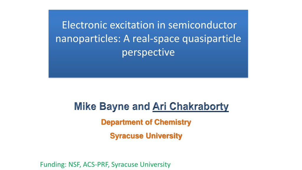
1. Electronic excitation in semiconductor nanoparticles: A real-space quasiparticle perspective Department of Chemistry Syracuse University Funding: NSF, ACS-PRF, Syracuse University

2. Overview of this talk Objective: To describe electron-hole screening without using unoccupied states Motivation: Calculation of unoccupied states are expensive. Judicious elimination of these states can lead to faster algorithm (e.g. WEST method by Galli et al.) Strategy: Treating electron correlation in real-space representation by using explicitly correlated operators Chemical applications: The developed method was used for calculations of optical gap and exciton binding energies

3. Charge-neutral excitation energy Matrix equation for excitation energies A B B A x y 1 0 0 -1 x y = * * Electron-hole interaction kernel (Keh) = + = eh ia jb eh ia jb ( ) ia jb A K ia jb B K , , , , ij ab a i Can be obtained using linear-response (LR-TDDFT), MBPT (BSE), equation-of-motion methods (EOM-CC, EOM-GF), CIS, ADC, Two important considerations: [1] Choice of 1-particles basis functions [2] Choice for treating e-e correlation

4. Effective single-particle Hamiltonian Non-interaction system Interacting system N = N eff( ) h H i = eff( ) v W V i 0 ee i i 2 N = = + + 2 ( , ) w i j h v v W eff ext eff 2 m i j Can be: { , } = + , , , , v v v MBPT v v model v H H W eff HF KS ps 0 = = = 0 0 | | |0 | H H E E E |0 = |0 H E 0 0 0 0 n a i a i | | H E n n n 0 = E = 0 0 0 n 0 0 E E 0 0 n n n = + (?) (?) (?) + + 0 Goal of today s talk: 0 0 n n

5. Definitions: Correlation operator Intermediate normalization condition = = 0| 1 a i | 1 0 n Electron-electron correlated is treated by operators that are local in real-space representation = x x ( ) ( x x x | | ' ') G G 0, 0, n n = = | |0 G a i | | G 0 0 n n G is a two-body operator and is represented by a linear combination of Gaussian-type geminal functions N N = g = 2 2 k 0,( , ) n i j G g / 12 r d (1,2) g b e 0, n k i j = 1 k

6. Definitions: Correlation operator Intermediate normalization condition = = 0| 1 a i | 1 0 n

7. Definitions: Correlation operator Intermediate normalization condition = = 0| 1 a i | 1 0 n Electron-electron correlated is treated by operators that are local in real-space representation = = | |0 G a i | | G 0 0 n n = x | ' x ( ) ( x x x | ') G G 0, 0, n n

8. Definitions: Correlation operator Intermediate normalization condition = = 0| 1 a i | 1 0 n Electron-electron correlated is treated by operators that are local in real-space representation = = | |0 G a i | | G 0 0 n n = x | ' x ( ) ( x x x | ') G G 0, 0, n n G is a two-body operator and is represented by a linear combination of Gaussian-type geminal functions N N = g = 2 2 k 0,( , ) n i j G g / 12 r d (1,2) g b e 0, n k i j = 1 k See also: geminal correlator (Rassolov et al.), NEO-XCHF (Hammes-Schiffer et al.), geminal MCSCF (Varganov & Martinez), trans-correlated Hamiltonian, Jastrow functions in VMC

9. Connection to Configuration Interaction (CI) N CI = kc Configuration interaction (CI): CI k k { }: finite number of independly optimizable coefficients kc = G Explicitly correlated wave function: 0 G = = | | | | | | G G G 0 0 0 k k k k = = 0 0 k k 1 G k c (must be a functional of G) The explicitly correlated wave function is an infinite-order CI expansion with constrained CI coefficients

10. Electron-hole interaction kernel The excitation energies for the interacting and non- interacting system are related by the W operator = = + a i | | E E H W 0 n n + 0| | H + W 0 0 0 = 0 0 a i | | 0| | W W 0 0 n n n

11. Electron-hole interaction kernel The excitation energies for the interacting and non- interacting system are related by the W operator = = = + a i | | E E H W 0 n n + 0| | H + W 0 0 0 0 0 a i | | 0| | W W 0 0 n n n Expressing in terms of non-interacting states using (G) = + 0 0 a i a i | | 0| |0 WG WG 0 0 n n n

12. Electron-hole interaction kernel The excitation energies for the interacting and non- interacting system are related by the W operator = = = + a i | | E E H W 0 n n + 0| | H + W 0 0 0 0 0 a i | | 0| | W W 0 0 n n n Expressing in terms of non-interacting states using (G) = + 0 0 a i a i | | 0| |0 WG WG 0 0 n n n Expressing in term of vacuum expectation value = + 0 0 0|{ } { }| i 0 0 | | 0 i a WG a WG 0 0 n n n Can be simplified using diagrammatic techniques

13. Contribution from the linked terms 0|{ } WG a i i a { }|0 n Only fully contracted terms have non-zero contribution to this term (Wick s theorem) The set of all resulting Hugenholtz diagrams, can be factored into sets of linked and unlinked diagrams Subset #1: All linked diagrams (all vertices are connected) Subset #2: All unlinked diagrams = + 0|{ } { }| i 0 0|{ } { }| i 0 0| |0 i a WG a i a WG a WG n n L n Because (algebraically): = 0|{ }{ }| 0 1 i a a i = 0|{ }| i 0 0 (normal ord ered) a Bayne, Chakraborty, JCTC, ASAP (2018)

14. Contribution from the linked terms 0|{ } WG a i i a { }|0 n Only fully contracted terms have non-zero contribution to this term (Wick s theorem) The set of all resulting Hugenholtz diagrams, can be factored into sets of linked and unlinked diagrams Subset #1: All linked diagrams (all vertices are connected) Subset #2: All unlinked diagrams Unlinked diagrams in excited state are exactly canceled by the ground state contributions = 0|{ } { }| i 0 0| | 0 0|{ } { } |0 i a W G a W G i a WG a i n n n L (Important point used in the next slide) Bayne, Chakraborty, JCTC, ASAP (2018)

15. Elimination of unlinked diagrams Adding zero to the expression = + + 0 0 0|{ } { }| 0 0| | 0 0 | |0 0| | 0 i a WG a i W G WG W G 0 0 n n n n n Only linked terms contribute in the following expression = 0|{ } { }| i 0 0| |0 0|{ } { }|0 i a WG a WG i a WG a i n n n L Expression for the excitation energy = + + 0 0 0|{ } { }| i 0 0| ( ) |0 i a WG a W G G 0 0 n n n L n Depends on particle-hole states Depends only on occupied states

16. Generalized Hugenhotlz vertices N N N N N = = + + ( , ) ( , ) ( , ) i j ( , , ) i j k ( , , , i j k l ) WG w i j g i j n n n n n i j i j i j i j i j k l WG = + + 2 3 4 n Product of two two-body operators generates 2, 3, and 4-body operators from 2-bo y d ve rtex ( ) 2

17. Contributing diagrams to the excitation energy

18. Contributing diagrams to the excitation energy Key result: Only connected diagrams contribute to the exciting energy and electron-hole interaction kernel Bayne, Chakraborty, JCTC, ASAP (2018)

19. Contributing diagrams to the excitation energy U U = , e h (effective 1-body) = K eh (effective 2-body)

20. Contributing diagrams to the excitation energy Contribution from different treatment of e-e correlation for ground and excited state wave function = = | |0 G a i | | G 0 0 n n = + + 0| ( ) |0 W G G D D D 0 19 20 21 n Impacts excitation energy Does not impact electron-hole interaction kernel Is zero if Gn = G0

21. Contributing diagrams to the excitation energy U U = , e h Effective 1-body (quasi) electron and hole operators Renormalizes quasiparticle energy levels due to e-e correlation Depends only on excited-state correlation operator Gn Impacts excitation energy Does not impact electron-hole interaction kernel

22. Contributing diagrams to the excitation energy = K eh It is an 2-particle operator that simultaneous operate on both (quasi) electron and hole states The loops represent renormalization of 3- and 4-body operators as effective 2-body operators All diagrams contribute to the electron-hole interaction kernel Depends only on excited-state correlation operator Gn 0 n G K = (eh screening is a consequence of ee correlation) = 0 eh

23. Interpretation of the closed-loops diagrams = K eh Closed-loops represent summation over occupied-state They represent effective 2-body operators generated from a 4-body operator by treating the additional coordinates at mean-field level

24. Interpretation of the closed-loops diagrams = K eh Closed-loops represent summation over occupied-state They represent effective 2-body operators generated from a 4-body operator by treating the additional coordinates at mean-field level = = N N N N N + + ( , ) ( , ) ( , ) i j ( , , ) i j k ( , , , i j k l ) WG w i j g i j n n n n n i j i j i j i j i j k l 1 4! = (3) (4) | (1,2,3,4)| (3) ( 4) i j n i j A , o cc i j

25. Just-in-time (JIT) source code generation = 0| { }... r |0 I h X X p q s 1 2 Y Y 1 2 pqrs pqrs Numerically zero mo integrals are eliminated Non-unique values are mapped to unique terms All non-zero & unique mo integerals are assigned a unique id The unique id of the mo integrals are used to consolidate terms in the reduction step Many-to-one map Key point: Incorporating molecular integrals in the reduction step

26. Computer assisted Wicks contraction The strings of second quantized operators were evaluated using generalized Wick s theorem Strategy#1: All contractions are performed computationally Strategy#2: Contractions are performed diagrammatically and the implementation is done computationally

27. Just-in-time (JIT) source code generation Disadvantages: Source code is generated every time the mo integrals are updated (new system and change of basis) Can be impractical for large codes that have long compilation time Advantages: The generated source code is optimized for the specific system Can reduce the overall memory footprint

28. Chemical application using first-order diagrams Bayne, Chakraborty, JCTC, ASAP (2018)

29. Application to chemical systems (1,2) (1, K w g = Excitation energies in small molecules and clusters G ( ) eh I 2)( G = 1 = ) P 12 0 , n approximations: = ( eh , ) ( e,h ) II III II III 0 K U [this work] [GW/BSE] [this work] [EOM-CCSD] 0 0 n n 0 0 n n System Energy difference in eV System Energy difference in eV Ne 0.06 Cd6Se6 Cd20Se19 0.04 (Ref. 1 & 3) H2O 0.03 -0.04 (Ref. 2 & 3) Results from this work show reasonable agreement with many-body methods that use unoccupied states 1 Noguchi, Sugino, Nagaoka, Ishii, Ohno, JCP, 137, 024306 (2012) 2 Wang, Zunger, PRB, 53, 9579 (1996) 3 Bayne, Chakraborty, to be submitted (this work) Bayne, Chakraborty, JCTC, ASAP (2018)

30. Exciton binding energies in CdSe clusters Conduction band Exciton binding (EBE) gap Quasiparticle energy gap 1st exciton level Optical absorption (OA) gap Valence band

31. Exciton binding energies in CdSe quantum dots E = 0 0 binding 0 n n

32. Exciton binding energies in CdSe quantum dots E = 0 0 binding 0 n n experiment This work theory

33. Summary It was shown that the electron-hole interaction kernel (eh- kernel) can be expressed without using unoccupied states. The derivation was performed using a two-body correlation operator which is local in real-space representation. Using diagrammatic techniques, it was shown that the eh- kernel can be expressed only in terms of linked-diagrams. The derived expression provides a route to make additional approximations to the eh-kernel The 1st order approximation of eh-kernel was used for calculating electron-hole binding energies and excitation energies in atoms, molecules, clusters, and quantum dots.

34. Title here

35. Deformation potential: Which basis? 0 = + h h Space-filling basis functions v def Examples: plane-waves, real-space grid, distributed Guassian functions, Harmonic osc. basis, particle-in-box basis Both deformed and reference Hamiltonian use identical basis functions Atom-centered basis functions Deformed and reference Hamiltonian use different basis functions We transform into the eigenbasis of the reference Hamiltonian

36. Transformation to ref. eigenbasis-I Step #1: Get quantities from the converged SCF calculation on reference structure = 0 0 0 0 0 F C S C Step #2: Perform symmetric or orthogonal transformation such that the S matrix is diagonal in that basis X S X X F X = = 0 0 I F (single tilde transformation) 0 0 0 Step #3: Find the U matrix that diagonalizes the transformed Fock matrix (double tilde transformation) = 0 0 ] 0 0 0 F U F U [ The U0 matrix is the matrix needed to transform operators in the eigenbasis of the reference structure

37. Transformation to ref. eigenbasis-II Step #4: Get quantities from the converged SCF calculation on the deformed structure = F C S C Step #5: Perform orthogonal transformation = = 0 X S X X F X I F 0 Step #6: Transform the Fock in the eigenbasis of the reference Hamiltonian = 0 ] 0 F U F U [ Step #7: Calculate the deformation potential = 0 V F F def

38. Info#: Contributing diagrams to the excitation energy N N = = ( ) ( , ) ( , i j ) ( , ) g i j G G g i j g 0 0 n n i j i j N N N N N = = + + ( 0) ( , ) w i j ( , ) ( , ) i j ( , , ) i j k ( , , , i j k l ) W G G g i j n n n n i j i j i j i j i j k l 1 2 N = 0| ( )|0 | (1 )| W G G 1 2 i i P 1 2 i i 0 2 12 n 1 2 i i 1 3! 3 ! N + ( 1) p | | 1 2 3 i i i P 1 2 3 i i i k 3 k = 1 1 2 3 i i i k 1 4! 4! N + ( 1 p | ) | 1 2 3 4 i i i i P i 2 3 4 i i i k 4 1 k = 1 1 2 3 4 i i i i k

39. Info#: Determination of geminal parameters For quantum dots, G was obtained from parabolic QD = + + + H T T V harm V model e h eh | | G H G mi n model model G e h e h | | G G G e h e h = G model G G G 0 n n For small molecules and clusters, G was obtained varaitionally 0| 0| |0 |0 G H G G G min G 0 G = G G 0 n

40. If we are ready to admit unoccupied states Phys. Rev. A89, 032515 (2014) Challenge: Avoiding 3, 4, 5, 6-particle integrals M Step 1: Project the correlation function in a finite basis = = | | E G HG G H G 0 0 0 0 k kk k ' kk M Step 2: Write the energy expression term of diagrams = + + + E D D D 1 2 36 kk M M = + + + + + lim M E D D D D Step 3: Obtain a renormalized 2-body operator by performing infinite-order summation over a subset of diagrams 1 10 11 36 kk kk 1 ( ) ( ) g r 12 r g r 12 12

41. Partial infinite-order diagrammatic summation M lim M D k All diagrams are added to infinite order = k XCHF E M lim M D k k + + M M lim M D D k k Some diagrams are added to infinite order = k k PCTH-PIOS E M M lim M D D k k k k M = D k k PCTH E All diagrams are added to finite order M D k k

42. Info#: Summation over intermediate particle-hole states Phys. Rev. A89, 032515 (2014) , , , a b c d = 42

43. Comparison of the three methods Infinite number of terms Infinite number of terms Finite number of terms c c c 10 9c 8c 7c 6c 5c 4c 3c 10 9c 8c 7c 6c 5c 4c 3c 10 9c 8c 7c 6c 5c 4c 3c Unconstrained optimization over infinite domain Unconstrained optimization over finite domain Constrained optimized over infinite domain 0| | G i 2c 2c 2c 1c 1c 1c exact FCI XCHF ic Infinite and independent ic Infinite and dependent ic Finite and independent

44. Ground state energy of helium atom 3 Key Points FCI - multi-determinant minimization. XCHF - single determinant minimization. XCHF gives lower energy than FCI for all the basis sets shown. XCHF converges much faster with respect to size 1-particle basis 1. Elward, Hoja, Chakraborty Phys. Rev. A. 86, 062504 (2012) See also: Geminal augmented MCSCF for H2, QMC calculations on H2O Varganov and Martinez, JCP, 132, 054103 (2010) ; Xu and Jordan, JPCA, 114, 1365 (2010)

45. Electron-hole Hamiltonian = + + + + + + ext e ext h H T V V T V V V e ee h hh eh interaction term hole subsystem electronic subs + ystem = H H V Coulomb attraction term is responsible for electron-hole coupling 0 eh Configuration interaction (CI): Zunger, Efros, Sundholm, Wang, Bester, Rabani, Franceschetti, Califano, Bittner, Hawrylak, This talk: Explicitly correlated Hartree-Fock Many-body perturbation theory (MBPT): Baer, Neuhauser, Galli,... Quantum Monte Carlo method (QMC): Hybertsen, Shumway, GW+BSE: Louie,Chelikowsky, Galli, Rohlfing, Rubio, All-electron TDDFT/DFT: Prezhdo, Tretiak, Kilina, Akimov, Ullrich, Li, .