Understanding Sample Size and Effect Size in Medical Statistics

Slide Note

Explore the crucial aspects of power analysis, sample size determination, effect size estimation, and their interrelations in medical statistics. Learn how these components influence experimental design and decision-making in research studies. Discover the significance of adequately balancing sample size to detect effects and interpreting effect sizes for meaningful conclusions.

milena Follow

Uploaded on Jul 23, 2024 | 0 Views

Download Presentation

Please find below an Image/Link to download the presentation.

The content on the website is provided AS IS for your information and personal use only. It may not be sold, licensed, or shared on other websites without obtaining consent from the author. Download presentation by click this link. If you encounter any issues during the download, it is possible that the publisher has removed the file from their server.

E N D

Presentation Transcript

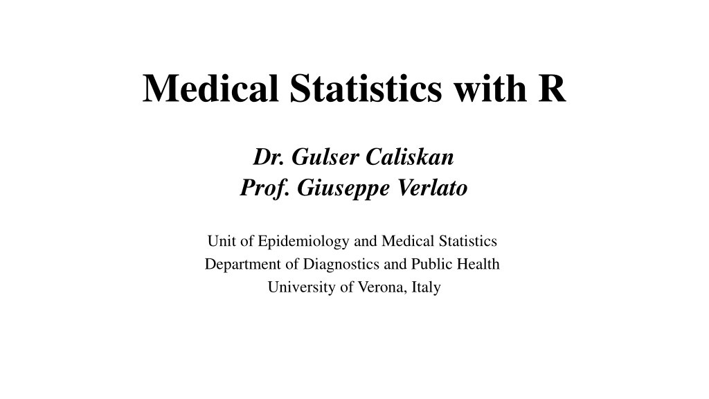
Medical Statistics with R Dr. Gulser Caliskan Prof. Giuseppe Verlato Unit of Epidemiology and Medical Statistics Department of Diagnostics and Public Health University of Verona, Italy

Power analysis is an important aspect of experimental design. It allows us to determine the sample size required to detect an effect of a given size with a given degree of confidence. Conversely, it allows us to determine the probability of detecting an effect of a given size with a given level of confidence, under sample size constraints. If the probability is unacceptably low, we would be wise to alter or abandon the experiment.

The following four quantities have an intimate relationship: Sample Size Effect Size Significance Level = P(Type I Error) = Probability of finding an effect that is not there Power = 1 - P(Type II Error) = Probability of finding an effect that is there Given any three, we can determine the fourth.

Sample Size How many In designing an experiment, a key question is: animals/subjects do I need for my experiment? Too small of a sample size can under detect the effect of interest in your experiment Too large of a sample size may lead to unnecessary wasting of resources and animals Goal: We strive to have enough samples to reasonably detect an effect if it really is there without wasting limited resources on too many samples.

Effect Size When a difference is statistically significant, it does not necessarily mean that it is big, important, or helpful in decision-making. It simply means you can be confident that there is a difference. To know if an observed difference is not only statistically significant but also important or meaningful, you will need to calculate its effect size. While the Power and Significance levels are usually set irrespective of the data, the effect size is a property of the sample data. It is essentially a function of the difference between the means of the null and alternative hypotheses over the variation (standard deviation) in the data.

How To Estimate Effect Size: 1. Use background information in the form of preliminary/trial data to get means and variation, then calculate effect size directly 2. Use background information in the form of similar studies to get means and variation, then calculate effect size directly 3. With no prior information, make an estimated guess on the effect size expected, then use an effect size that corresponds to the size of the effect Broad effect sizes categories are small, medium, and large Different statistical tests will have different values of effect size for each category

To interpret the resulting number, most social scientists use this general guide developed by Cohen: < 0.1 = Trivial Effect 0.1 - 0.3 = Small Effect 0.3 - 0.5 = Moderate Effect > 0.5 = Large Difference Effect

Effect Size Calculation within R As opposed to GPower, which allows you to enter details such as means and standard deviations into the program and it will calculate effect size for you, that is not the case for R Most R functions for sample size only allow you to enter effect size If you want to estimate effect size from background information, you ll need to calculate it yourself first

POWER ANALYSIS IN R The pwr package develped by St phane Champely, impliments power analysis as outlined by Cohen (1988). Some of the more important functions are listed below.

# Name of Test in R? Package Function 1 One Mean T-test Yes pwr.t.test pwr pwr 2 Two Means T-test Yes pwr.t.test 3 Paired T-test Yes pwr.t.test pwr pwr pwr pwr pwr 4 One-way ANOVA Yes pwr.anova.test 5 Single Proportion Test Yes pwr.p.test 6 Two Proportions Test Yes pwr.2p.test 7 Chi-Squared Test Yes pwr.chisq.test 8 Simple Linear Regression Yes pwr.f2.test pwr pwr pwr 9 Multiple Linear Regression Yes pwr.f2.test 10 Correlation Yes pwr.r.test 11 One Mean Wilcoxon Test Yes* pwer.t.test + 15% pwr pwr pwr pwr 12 Mann-Whitney Test Yes* pwer.t.test + 15% 13 Paired Wilcoxon Test Yes* pwer.t.test + 15% 14 Kruskal Wallis Test Yes* pwr.anova.test + 15% 15 Repeated Measures ANOVA Yes wp.rmanova WebPower WebPower 16 Multi-way ANOVA (1 Category of interest) Yes wp.kanova 17 Multi-way ANOVA (>1 Category of interest) Yes wp.kanova WebPower WebPower 18 Non-Parametric Regression (Logistic) Yes wp.logistic 19 Non-Parametric Regression (Poisson) Yes wp.poisson WebPower 20 Multilevel modeling: CRT Yes wp.crt2arm/wp.crt3arm WebPower 21 Multilevel modeling: MRT Yes wp.mrt2arm/wp.mrt3arm WebPower Simr & lme4 22 GLMM Yes^ n/a *-parametric test with non-parametric correction ^-detailed in future Module

ONE MEAN T-TEST This tests if a sample mean is any different from a set value for a normally distributed variable. pwr.t.test(d = , sig.level = , power = , type = c("two.sample", "one.sample", "paired")) Effect size calculation Cohen s D = (M2-M1)/SD M2=Mean 2 M1=Mean 1 SD =Standard deviation d=Effect Size sig.level=Significant Level power=Power of Test type=Type of Test

EXERCISES:

a year for college freshman is greater than zero. Guessed a large effect size (0.8), and used one-tailed test You are interested in determining if the average weight change in

POWER OF TWO-SAMPLE T TEST It is generally assumed that the variance is the same in the two groups, that is, using the Welch procedure is not considered. sizes are the same, since that gives the optimal power for a given total number of observations. In sample-size calculations, one usually assumes that the group

For t-tests, use the following functions: pwr.t.test(n = , d = , sig.level = , power = , type = c("two.sample", "one.sample", "paired")) d=Effect Size sig.level=Significant Level power=Power of Test type=Type of Test

where n is the sample size, d is the effect size, and type indicates a two- sample t-test, one-sample t-test or paired t-test. If you have unequal sample sizes, use pwr.t2n.test(n1 = , n2= , d = , sig.level =, power = ) where n1 and n2 are the sample sizes.

For t-tests, the effect size is assessed as Cohen s D = (M2-M1)/SDpooled M2=Mean 2 M1=Mean 1 SDpooled =Pooled standard deviation SDpooled= ((SD12+ SD22)/2) Cohen suggests that d values of 0.2, 0.5, and 0.8 represent small, medium, and large effect sizes respectively.

EXERCISES : Calculate the sample size for the following scenarios (with =0.05, and power=0.80):

You are interested in determining if the average daily caloric intake different between men and women. found the average caloric intake for males to be 2350.2 (SD=258), while females had intake of 1872.4 (SD=420). You collected trial data and Effect size = (MeanH1-MeanH0)/ SDpooled =(2350.2-1872.4)/ ((2582+ 4202)/2) = 477.8/348.54 = 1.37

You are interested in determining if the average protein level in blood different between men and women. trial data on protein level (grams/deciliter). You collected the following Effect size = (MeanH1-MeanH0)/ SDpooled =(4.59-4.98)/ ((2.582+ 2.882)/2) = -0.14

PAIRED T-TEST This tests if a mean from one group is different from the mean of another group, where the groups are dependent (not independent) for a normally distributed variable. Pairing can be leaves on same branch, siblings, the same individual before and after a trial, etc. Effect size calculation Cohen s D = (M2-M1)/SDpooled M2=Mean 2 M1=Mean 1 SDpooled =Pooled standard deviation SDpooled= ((SD12+ SD22)/2) For t-tests; 0.2=small, 0.5=medium, and 0.8 large effect sizes

EXERCISES: Calculate the sample size for the following scenarios (with =0.05, and power=0.80):

You are interested in determining if heart rate is higher in patients after a doctor s visit compared to before a visit. following trial data and found mean heart rate before and after a visit. You collected the Effect size = (MeanH1-MeanH0)/ SDpooled =(98.1-85.4)/ ((26.82+ 27.22)/2) =12.7/27 = 0.47

You are interested in determining if metabolic rate in patients after surgery is different from before surgery. found a mean difference of 0.73 (SD=2.9). Effect size = (MeanH1-MeanH0)/ SD =(0.73)/ 2.9 = 0.25 You collected trial data and

ANALYSIS OF VARYANS (ANOVA) For a one-way analysis of variance use pwr.anova.test(k = , n = , f = , sig.level = , power = ) where k is the number of groups and n is the common sample size in each group. k=Number of Groups f=Effect Size sig.level=Significant Level power=Power of Test

For a one-way ANOVA effect size is measured by f where

EXERCISES: =0.05, and power=0.80): Calculate the sample size for the following scenarios (with

You are interested in determining if there is a difference in white blood cell counts between 5 different medication regimes. Guessed a medium effect size (0.25) and 5 groups n = 39.15 -> 40 samples per group (200 total)

POWER OF COMPARISONS OF PROPORTIONS populations and have to decide the number of persons to sample from each population. That is, you plan to perform a comparison of two binomial distributions as described in previous using prop.test or chisq.test. Suppose you wish to compare the morbidity between two

When comparing two proportions use pwr.2p.test(h = , n = , sig.level =, power = )

where h is the effect size and n is the common sample size in each group.

EXERCISES: Calculate the sample size for the following scenarios (with =0.05, and power=0.80):

You are interested in determining if the expected proportion (P1) of students passing a stats course taught by psychology teachers is different than the observed proportion (P2) of students passing the same stats class taught by biology teachers. You collected the following data of passed tests. P1=7/10=0.70, P2=6/10=0.60 h= 2*asin(sqrt(0.60))-2*asin(sqrt(0.70))=-0.21

You are interested in determining of the expected proportion (P1) of female students who selected YES on a question was higher than the observed proportion (P2) of male students who selected YES. The observed proportion of males who selected yes was 0.75. Guess that the expected proportion (P1) =0.85 h= 2*asin(sqrt(0.85))-2*asin(sqrt(0.75))=0.25

CHI-SQUARED TEST Extension of proportions test, which asks if table of observed values are any different from a table of expected ones. Also called Goodness-of-fit test. For w-tests: 0.1=small, 0.3=medium, and 0.5 large effect sizes

EXERCISES: Calculate the sample size for the following scenarios (with =0.05, and power=0.80):

You are interested in determining if the ethnic ratios in a hospital differ by gender. You collect the following employees. trial data from 200 2(Chi-squared)= (O-E)2/E = (60-62.5)2/62.5 + (25-23)2/23 + (1-6)2/6 + (14-8.5)2/8.5=0.10 + 0.17 + 4.17 + 3.56 = 8 w = ( 2/(n*df))= (8/(200*3))=0.115

NON-PARAMETRIC T-TESTS Versions of the t-tests for non-parametric data. One Mean Wilcoxon: sample mean against set value Mann-Whitney: two sample means (unpaired) Paired Wilcoxon: two sample means (paired) There aren t any R packages that had useful non-parametric t-tests but suggested using the parametric + 15% approach.