Understanding Limit Cycles and Bifurcations in Dynamical Systems
Explore the stability of limit cycles and bifurcations in dynamical systems through examples like the Holling-Tanner model. Discover the significance of stable limit cycles and the role of Liapunov functions in forbidding closed orbits. Delve into the intriguing behavior of trajectories in bottleneck regions and the influence of eigenvalues of the Jacobian. Uncover the nonlinearity and complexity inherent in self-sustained oscillations in various systems.

Download Presentation

Please find below an Image/Link to download the presentation.
The content on the website is provided AS IS for your information and personal use only. It may not be sold, licensed, or shared on other websites without obtaining consent from the author. Download presentation by click this link. If you encounter any issues during the download, it is possible that the publisher has removed the file from their server.
E N D
Presentation Transcript
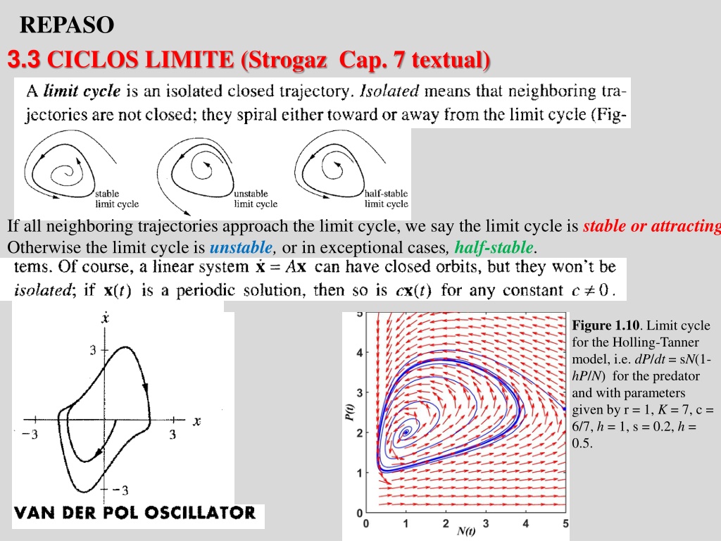
REPASO 3.3 CICLOS LIMITE (Strogaz Cap. 7 textual) If all neighboring trajectories approach the limit cycle, we say the limit cycle is stable or attracting Otherwise the limit cycle is unstable, or in exceptional cases, half-stable. Figure 1.10. Limit cycle for the Holling-Tanner model, i.e. dP/dt = sN(1- hP/N) for the predator and with parameters given by r = 1, K = 7, c = 6/7, h = 1, s = 0.2, h = 0.5.
Stable limit cycles are very important scientifically-they model systems that exhibit self-sustained oscillations. In other words, these systems oscillate even in the absence of external periodic forcing. Of the countless examples that could be given, we mention only a few: the beating of a heart; daily rhythms in human body temperature and hormone secretion; chemical reactions that oscillate spontaneously; and dangerous self-excited vibrations in bridges and airplane wings In each case, there is a standard oscillation of some preferred period, waveform, and amplitude. If the system is perturbed slightly, it always returns to the standard cycle. Limit cycles are inherently nonlinear phenomena; they can't occur in linear systerns.
If a Liapunov function exists, then closed orbits are forbidden Unfortunately, there is no systematic way to construct Liapunov functions. Divine inspiration is usually required, although sometimes one can work backwards. Sums of squares occasionally work, as in the following example.
ogy. For details, see Perko (1991), Coddington and Levinson (1955), Hurewicz (1958), or Cesari (1963).
In the x-direction we see the bifurcation behavior discussed in Section 3.1, while in the y-direction the motion is exponentially damped. Figure 8.1.1 Even after the fixed points have annihilated each other, they continue to influence the flow-as in Section 4.3, they leave a ghost, a bottleneck region that sucks trajectories in and delays(*) them before allowing passage out the other side. (*): Se puede ver que the time spent in the bottleneck generically increases as ( c)-1/2.
Es ms claro visualizarlo en 3 dimensiones: Para los diferentes valores del par metro tenemos diferentes puntos de equilibrio y al variar el par metro en un rango va describiendo una curva: presa presa S bitamente, para un valor del par metro se pierde la estabilidad y comienza un ciclo de oscilaci n, esa es una bifurcaci n de Hopf, como muestra la figura.
Vimos que un modelo de Lotka-Volterra realista (con respuesta Holling II o III) lo podemos pensar como el LBJ de pastoreo en el que el consumo incluye a la densidad del predador nos ayuda a entender esto. Diferentes par metros pueden afectar la estabilidad. Dos de particular inter s en la pr ctica son: la productividad de la presa y la eficiencia del consumidor. La productividad a menudo depende de la riqueza de nutrientes que afecta la capacidad de carga de la poblaci n de alimentos (K). Puede verse en los gr ficos que un aumento en K puede cambiar un sistema de estable (panel a) a inestable (panel b). sta es la famosa paradoja del enriquecimiento. El momento crucial es cuando el punto de inflexi n de la derecha en la curva de equilibrio plegada de la presa cruza a la l nea de equilibrio horizontal del consumidor. Esto cambia el comportamiento asint tico del sistema de forma cualitativa: Un punto estable se convierte en un ciclo. Este punto crucial de desestabilizaci n se conoce como "bifurcaci n de Hopf".
3.5 COMPETENCIA Y PRINCIPIO DE EXCLUSIN COMPETITIVA (sigo textualFort 2020) 1.4.1 A descriptive or phenomenological model Lotka (1925) and Volterra (1926) independently proposed the simplest dynamical system for modeling two-species competition using extensions of the logistic equation. The Lotka-Volterra competition model is an interferencecompetition model: two species are assumed to diminish each other's per capita growth rate by direct interference. But the model does not specify neither the limiting resource(s) the two species are competing for (nutrients, light, shelter, nesting sites, whatever), nor the mechanism of competition. Thus it is a descriptive or phenomenological model of competition rather than a mechanistic model. We begin by assuming that two species, with populations densities N1and N2, each grow logistically in the absence of the other. Each species has a per capita growth rate that decreases linearly with population size, + = K En realidad 12 corresponde a la competencia inter-espec fica; la log stica incluye competencia intra-espec fica. Noten que estamos asumiendo 11= -1. where the competition coefficients 12 is a positive parameter measuring the per capita effect of sp. 2 on the abundance of sp. 1 ( ) t ( ) ( ) dN t d N t N t r ( ) 1 , N t 1 1 12 2 1 1 1 + K ( ) ( ) ( ) dN t d N t N t r = ( ) 1 . N t 2 t 2 21 1 2 2 2
1.4.2 Stable equilibrium: Competitive exclusion or species coexistence? To understand the dynamics and equilibria of this model, let us start by finding the nullclines. Both the nullclines and the equilibrium solutions are found by setting either the riNiterms or the [1 (Ni ijNj)/Ki] terms equal 0. The nullclines for N1 are: N1 = 0 (1.40a) and N1 = K1 12N2 (1.40b) Likewise, the nullclines for N2 are: and N2 = 0 (1.40c) N2 = K2 21N1 (1.40d) As with predator prey models, the N1 and N2axes are the extinction nullclines for the other species.
Regarding the combination of the two inclined nullclines, there are four different possibilities: I. If each intercept of the sp. 2 nullcline, N1 = K2/ 21 and N2 = K2, is greater than the corresponding intercept of the sp. 1, N1 = K1 and N2 = K1/ 12, i.e. K2/ 21 > K1 i.e. K2/ 21 > K1 and K2 > K1/ 12, which implies that 12>K K1/K K2, 21 < K K2/K K1then N2 excludes N1. II. If each intercept of the sp. 1 nullcline is greater than the corresponding intercept of sp. 2 nullcline, i.e. K1 > K2/ 21 and K1/ 12 > K2, which implies that 12<K K1/K K2, 21 > K K2/K K1, then N1 excludes N2. III. If the two nullclines cross in such a way that K1 > K2/ 21 and K2 > K1/ 12, which implies that 12>K K1/K K2, 21 > K K2/K K1 i.e. both species are strong competitors against the other, Then the vector field shows that either species can displace the other to extinction, depending on the initial conditions. That is, the two equilibria (K1,0) and (0,K2), corresponding to the exclusion of one species, are now stable nodes IV. Finally, if both species are weak competitors as defined by 12<K K1/K K2, 21 < K K2/K K1 , the vector field now shows that there is a coexistence equilibrium and that the equilibria (K1, 0) and (0, K2)are now unstable saddle points
Thus the four possible equilibria are: * * 0, = = = * 0 (1.42a) = , * 0 (1.42b) * N = K N N N N K 1 2 = * N 1 1 2 (1.42c) 1 2 2 K K K K = = * N , * (1.42d) N 1 12 2 2 21 1 1 2 1 1 12 21 12 21 The above four possible competitive situations, defined by the relative positions of the nullclines, are summarized in Table 1.1. Effect of species 2 on species 1 Effect of species 1 on species 2 Weak: < K1/ Coexistence Strong: > K1/ Species 2 always displaces species 1, Weak: < K2/ equilibrium at K K K K , 1 12 2 2 21 1 equilibrium at (0,K2) 1 1 12 21 12 21 Strong: > K2/ Species 1 always displaces species 2, Winner depends on initial conditions, equilibrium at (K1,0) if N1(0) > N2(0), equilibrium at (K1,0) if N1(0) < N2(0), equilibrium at (0,K2)
We can conclude form Table 1.1 that whenever at least one of the two interspecific effects is strong, i.e. stronger than intraspecific competition, we end up with competitive exclusion of one species. Only in case IV, where both interspecific effects were weak relative to intraspecific effects, did the two competing species coexist. This forms the basis for Gause's Principle (Gause, 1934) aka the Principleof Competitive Exclusion. This principle states that, two species competing for the very same ecological niche cannot coexist. This leads either to the extinction of the weaker competitor or to an evolutionary or behavioral shift toward a different ecological niche. Thus it begs the question: just how similar can the two niches be in order the two species manage to coexist? We will revisit this question in the second part of this book when dealing with niche theory.
Lets illustrate this concept using birds. The idea is that the beak size determines what a bird can eat. The beak size determines the utilization ability of resources (e.g. seeds). For a given beak size, a bird species can optimally feed on a particular size of seed, and its feeding ability drops off for seeds that depart from this size. Niche overlap hypothesis: the larger the overlapping of 2 distributions, the strongest the competition between the corresponding pair of species.


, Coddington")
")