Understanding Measures of Central Tendency in Data Analysis
Measures of central tendency, including mean and median, play vital roles in summarizing and interpreting data. The mean is the average calculated by summing all values and dividing by the count, while the median is the middle score when data is arranged in order. These measures provide insight into the typical value and help in making informed decisions based on data distributions.

Download Presentation

Please find below an Image/Link to download the presentation.
The content on the website is provided AS IS for your information and personal use only. It may not be sold, licensed, or shared on other websites without obtaining consent from the author. Download presentation by click this link. If you encounter any issues during the download, it is possible that the publisher has removed the file from their server.
E N D
Presentation Transcript
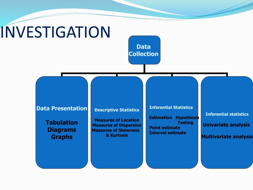
INVESTIGATION Data Collection Inferential Statistics Data Presentation Descriptive Statistics Inferential statistics Estimation Hypothesis Measures of Location Measures of Dispersion Measures of Skewness & Kurtosis Tabulation Diagrams Graphs Testing Univariate analysis Point estimate Interval estimate Multivariate analysis
Summary Measures Describing Data Numerically Central Tendency Quartiles Variation Shape Arithmetic Mean Range Skewness Median Interquartile Range Mode Variance Geometric Mean Standard Deviation Harmonic Mean 2
Measures of Central Tendency A statistical measure that identifies a single score as representative for an entire distribution. The goal of central tendency is to find the single score that is most typical or most representative of the entire group There are three common measures of central tendency: the mean the median the mode 3
Calculating the Mean Calculate the mean of the following data: 1 5 4 3 2 Sum the scores ( X): 1 + 5 + 4 + 3 + 2 = 15 Divide the sum ( X = 15) by the number of scores (N = 5): 15 / 5 = 3 Mean = X = 3 4
Mean (Arithmetic Mean) (continue d) The most common measure of central tendency Affected by extreme values (outliers) 0 1 2 3 4 5 6 7 8 9 10 0 1 2 3 4 5 6 7 8 9 10 12 14 Mean = 5 Mean = 6 5
The Median The median is simply another name for the 50th percentile It is the score in the middle; half of the scores are larger than the median and half of the scores are smaller than the median 6
How To Calculate the Median Conceptually, it is easy to calculate the median Sort the data from highest to lowest Find the score in the middle middle = (N + 1) / 2 If N, the number of scores is even, the median is the average of the middle two scores 7
Median Example What is the median of the following scores: 10 8 14 15 7 3 3 8 12 10 9 Sort the scores: 15 14 12 10 10 9 8 8 7 3 3 Determine the middle score: middle = (N + 1) / 2 = (11 + 1) / 2 = 6 Middle score = median = 9 8
Median Example What is the median of the following scores: 24 18 19 42 16 12 Sort the scores: 42 24 19 18 16 12 Determine the middle score: middle = (N + 1) / 2 = (6 + 1) / 2 = 3.5 Median = average of 3rd and 4th scores: (19 + 18) / 2 = 18.5 9
Median Not affected by extreme values 0 1 2 3 4 5 6 7 8 9 10 0 1 2 3 4 5 6 7 8 9 10 12 14 Median = 5 Median = 5 In an ordered array, the median is the middle number If n or N is odd, the median is the middle number If n or N is even, the median is the average of the two middle numbers 10
Measures of Central Tendency Mean the most frequently used but is sensitive to extreme scores e.g. 1 2 3 4 5 6 7 8 9 10 Mean = 5.5 (median = 5.5) e.g. 1 2 3 4 5 6 7 8 9 20 Mean = 6.5 (median = 5.5) e.g. 1 2 3 4 5 6 7 8 9 100 Mean = 14.5 (median = 5.5)
Mode Value that occurs most often Not affected by extreme values Used for either numerical or categorical data There may be no mode There may be several modes 0 1 2 3 4 5 6 0 1 2 3 4 5 6 7 8 9 10 11 12 13 14 No Mode Mode = 9 12
The Shape of Distributions Distributions can be either symmetrical or skewed, depending on whether there are more frequencies at one end of the distribution than the other. ? 13
Symmetrical Distributions A distribution is symmetrical if the frequencies at the right and left tails of the distribution are identical, so that if it is divided into two halves, each will be the mirror image of the other. In a symmetrical distribution the mean, median, and mode are identical. 14
Distributions Bell-Shaped (also known as symmetric or normal ) skew6 Skewed: positively (skewed to the right) it tails off toward larger values negatively (skewed to the left) it tails off toward smaller values 15
Skewed Distribution Few extreme values on one side of the distribution or on the other. Positively skeweddistributions: distributions which have few extremely high values (Mean>Median) Negatively skewed distributions: distributions which have few extremely low values(Mean<Median) 16
Positively Skewed Distribution GOVT INVESTIGATE WORKERS ILLEGAL DRUG USE Mean=1.13 500 400 Median=1.0 300 200 Frequency 100 Std. Dev = .39 Mean = 1.1 N = 474.00 0 1.0 2.0 3.0 4.0 GOVT INVESTIGATE WORKERS ILLEGAL DRUG USE 17
Negatively Skewed distribution FAVOR PREFERENCE IN HIRING BLACKS 600 Mean=3.3 500 400 Median=4.0 300 200 Frequency 100 Std. Dev = .98 Mean = 3.3 N = 908.00 0 1.0 2.0 3.0 4.0 FAVOR PREFERENCE IN HIRING BLACKS 18
Choosing a Measure of Central Tendency IF variable is Nominal.. Mode IF variable is Ordinal... Mode or Median(or both) IF variable is Interval-Ratio and distribution is Symmetrical Mode, Median or Mean IF variable is Interval-Ratio and distribution is Skewed Mode or Median 19
EXAMPLE: x (1) 7,8,9,10,11 n=5, x=45, =45/5=9 (2) 3,4,9,12,15 n=5, x=45, =45/5=9 x x (3) 1,5,9,13,17 n=5, x=45, =45/5=9 S.D. : (1) 1.58 (2) 4.74 (3) 6.32
Measures of Dispersion Or Measures of variability 21
Series I: 70 70 70 70 70 70 70 70 70 70 Series II: 66 67 68 69 70 70 71 72 73 74 Series III: 1 19 50 60 70 80 90 100 110 120 22
Measures of Variability A single summary figure that describes the spread of observations within a distribution. 23
Measures of Variability Range Difference between the smallest and largest observations. Interquartile Range Range of the middle half of scores. Variance Mean of all squared deviations from the mean. Standard Deviation Rough measure of the average amount by which observations deviate from the mean. The square root of the variance. 24
Variability Example: Range Marks of students 52, 76, 100, 36, 86, 96, 20, 15, 57, 64, 64, 80, 82, 83, 30, 31, 31, 31, 32, 37, 38, 38, 40, 40, 41, 42, 47, 48, 63, 63, 72, 79, 70, 71, 89 Range: 100-15 = 85 25
Quartiles Q1, Q2, Q3 divides ranked scores into four equal parts 25% 25% 25% 25% Q3 Q2 (median) Q1 (minimum) (maximum) 26
Quartiles: n+1 th 4 2(n+1) = 4 3(n+1) th 4 Q Q 1 = n+1 2 2 = th Q 3 = Inter quartile : IQR = Q3 Q1 27
Inter quartile Range The inter quartile range is Q3-Q1 50% of the observations in the distribution are in the inter quartile range. The following figure shows the interaction between the quartiles, the median and the inter quartile range. 28
Percentiles and Quartiles Maximum is 100th percentile: 100% of values lie at or below the maximum Median is 50th percentile: 50% of values lie at or below the median Any percentile can be calculated. But the most common are 25th (1st Quartile) and 75th (3rd Quartile) 30
Locating Percentiles in a Frequency Distribution A percentile is a score below which a specific percentage of the distribution falls(the median is the 50th percentile. The 75th percentile is a score below which 75% of the cases fall. The median is the 50th percentile: 50% of the cases fall below it Another type of percentile :The quartile lower quartile is 25th percentile and the upper quartile is the 75th percentile 32
Locating Percentiles in a Frequency Distribution 25% included N U M B E R O F r e q u e n c y P e r c e n t Va lid P e r c e n t C u m P e r c e n t F C H IL D R E N 0 2 3 4 5 6 7 E I G HT O T o ta l N A T o ta l Va lid u la tive here 25th percentile 50% included 50th percentile here 80th 80% included percentile here R MO R E 33
VARIANCE: Deviations of each observation from the mean, then averaging the sum of squares of these deviations. STANDARD DEVIATION: ROOT- MEANS-SQUARE-DEVIATIONS 34
Standard Deviation To undo the squaring of difference scores, take the square root of the variance. Return to original units rather than squared units. 35
Quantifying Uncertainty Standard deviation: measures the variation of a variable in the sample. Technically, N = = 2 ( ) s x x 1 i 1 N 1 i 36
Example: Data: X = {6, 10, 5, 4, 9, 8}; N = 6 Mean: X 2) X X 6 10 5 4 9 8 ( X X = X 42= = 7 X -1 3 -2 -3 2 1 1 9 4 9 4 1 6 N Variance: 2 ( ) X X 28 6 = = = 2 4.67 s N Standard Deviation: = s = = 2 . 4 67 . 2 16 s Total: 42 Total: 28
Calculation of Variance & Standard deviation Using the deviation & computational method to calculate the variance and standard deviation Example: 3,4,4,4,6,7,7,8,8,9 ; Given n=10; Sum= 60; Mean = 6 = 2 ( ) X X S n ) 6 4 ( + ) 6 4 ( + ) 6 4 ( + ) 6 6 ( + ) 6 7 ( + ) 6 7 ( + ) 6 + ) 6 + ) 6 + ) 6 2 2 2 2 2 2 2 2 2 2 3 ( 8 ( 8 ( 9 ( = S 10 40 = = = ; 0 . 2 var 4 S iance 10 X2 X 2 2 ( ) n X X = 3 4 4 4 6 7 7 8 8 9 9 S 2 n 16 16 16 36 49 49 64 64 81 2 10 ( 400 ) ( 60 ) = S 2 10 4000 3600 = S 100 = 0 . 4 S = = , 0 . 2 var 4 S iance Sum: 60 Sum: 400 38
WHICH MEASURE TO USE ? DISTRIBUTION OF DATA IS SYMMETRIC ---- USE MEAN & S.D., DISTRIBUTION OF DATA IS SKEWED ---- USE MEDIAN & QUARTILES 39


")