Understanding Urban Trip Distribution Modeling Methods
Urban trip distribution modeling involves processes like trip generation, path skimming, and impedance calculation, using methods like gravity models to determine travel patterns between zones. Factors such as trip productions, attractions, travel times, and friction factors play crucial roles in estimating the number of trips exchanged between different zones within an area.

Download Presentation

Please find below an Image/Link to download the presentation.
The content on the website is provided AS IS for your information and personal use only. It may not be sold, licensed, or shared on other websites without obtaining consent from the author. Download presentation by click this link. If you encounter any issues during the download, it is possible that the publisher has removed the file from their server.
E N D
Presentation Transcript
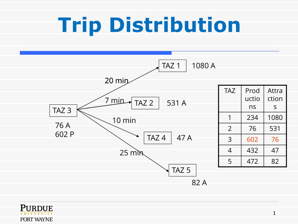
Trip Distribution TAZ 1 1080 A 20 min 20 min TAZ Prod uctio ns 234 76 602 432 472 Attra ction s 1080 531 76 47 82 7 min TAZ 2 531 A TAZ 3 1 2 3 4 5 10 min 76 A 602 P TAZ 4 47 A 25 min TAZ 5 82 A 1
Inputs and Outputs Input Trip generation - productions & attractions (balanced by purpose) Path skimming - travel times or impedances Travel times in form of matrix, each cell represents time it takes to travel from one TAZ to another Output of trip distribution model: trip table or OD matrix, each cell represents number of person trips between each zonal exchange 2
Impedance: Travel Time Matrix Trip Generation P & A per purpose TAZ Productions TAZ 1 2 3 4 5 Attractions 1 4 12 8 15 21 1 234 1080 2 6 3 9 23 14 2 76 531 3 20 7 4 10 25 3 602 76 4 12 18 8 4 17 4 432 47 5 24 19 23 15 8 5 472 82 Trip Distribution TAZ 1 2 3 4 5 Production 234 76 602 432 472 1816 1 199 2 15 2 16 2 35 25 12 3 1 3 147 350 78 19 8 4 330 90 4 6 2 5 369 90 7 5 1 1080 531 76 47 82 Attraction 3
Method: Gravity Model Adapted from Newton s Law of Gravitation Gravitation force = f(mass & distance between two objects) Applied to trip distribution Travel between two TAZs = f(relative attractiveness of TAZs & accessibility) Determines number of trips being exchanged between two TAZs Performed for all zonal interchanges in area 4
Gravity Model A F K Pi j A ij F ij K = T P j ij i j ij ij Tij Fij Tij = Trips from zone i to zone j Pi = Trip production in zone i Aj = Trip attraction in zone j Fij =Friction factor: Effect of travel time, distance & cost between zones i & j Kij = Socioeconomic factor Kij Aj 5
Friction Factor Fij Represent travel time of impedance in gravity model Express effects of spatial separation or accessibility on travel patterns Must be calibrated: frequency of travel from trip distribution matches frequency observed in travel surveys Assumed not to change for forecast year Higher as travel time decreases Differ by trip purposes HBW: largest, NHB: middle, HBO: smallest Greater friction factor or # of attractions compared to other TAZs means greater relative attractiveness of TAZ 6
Friction Factor Fij Power function ?, ? < 0 ???= ??? Exponential function ???= exp ? ???, ? < 0 Gamma function ???= ? ??? Coefficient Estimation for Gamma Functions (Source: NCHRP 365) Trip Purpose a HBW 28,507 HBO 139,173 NHB 219,113 ? exp ? ???, ? > 0,? < 0,? < 0 b c -0.020 -1.285 -1.332 -0.123 -0.094 -0.100 7
Intrazonal Travel Times Generally not produced by software Must be estimated Determines # of trips staying within TAZ Nearest neighbor technique: ???????= 0.5 ??????????????? Function of TAZ area & intrazonal speed TTintra intrazonal TT (min) ???????= 30 ???????+ ?????? TAZarea area of TAZ (mi2) Vintra intrazontal speed (mph) CBD: Vintra = 15 mph 8 Rural: Vintra = 30 mph
Kij Factor Accounts for socioeconomic linkages not accounted for by gravity model Accounts for variables other than travel time i-j TAZ specific factor If i-j pair has too many trips, use K-factor < 1.0 If i-j pair has too few trips, use K-factor > 1.0 K-factor = 0 prohibit trip Use with caution, decreases sensitivity of model to variables which may change over time 9
Trip Distribution, Example, Step 1 TAZ 1 1080 A 20 min 20 min TAZ Prod uctio ns 234 76 602 432 472 Attra ction s 1080 531 76 47 82 7 min TAZ 2 531 A TAZ 3 1 2 3 4 5 10 min 76 A 602 P TAZ 4 47 A 25 min TAZ 5 82 A 10
Calculate Friction Factors, Step 2 Travel time (min) Friction Factor 87 45 29 18 10 6 4 3 4 7 10 15 20 25 For TAZ 3: Attraction TAZ TT F 1 2 7 3 4 45 4 10 18 5 25 4 20 6 29 Intra-zonal travel time must be estimated since there is no network within zones 11
Calculate Attractiveness of Each TAZ, Step 3 ????= ?? ??? i = production TAZ, j = attraction TAZ Attract ion TAZ Aj 1 2 3 4 5 1,080 531 76 47 82 Fij 6 29 45 18 4 Aj*Fij 6,480 15,399 3,420 846 328 Kij not given assume Kij = 1 12
Calculate Relative Attractiveness of Each TAZ, Step 4 ?? ??? ?? ??? ???????= Attraction TAZ 1 2 3 4 5 Total Aj*Fij 6,480 15,399 3,420 846 328 26,473 6480 /26473 =0.2448 Attrel j 0.5817 0.1292 0.0319 0.0124 1.000 13
Distribute Productions to TAZs (apply Gravity Model), Step 5 ???= ?? ??????? P3 = 602 (total production of TAZ 3) Relative attractiveness 0.2448 TAZ Distributed Trips 1 147 2 0.5817 350 3 0.1292 78 4 0.0319 19 5 0.0124 8 Total 1.0000 602 Repeat 1 5 for each TAZ 14
Trip Distribution: First Iteration, Step 6 TAZ 1 1080 A 147 trips 350 trips TAZ 2 531 A TAZ 3 19 trips Intra-zonal 78 trips A TAZ 4 47 A TAZ 1 2 3 4 5 1 2 2 3 4 2 3 19 6 5 5 16 1 8 2 1 8 trips 199 35 147 330 369 15 12 78 4 7 25 350 90 90 TAZ 5 P 82 A 15
Adjust Attractions, Step 7 Compare # of attractions distributed to each TAZ # of attractions estimated from trip generation Adjust In subsequent iterations, # of attractions used in gravity model for each TAZ is adjusted based on whether gravity model over or under estimated trips in previous iteration Iterations continues until two (closely) match (typically 4 to 5 iterations required) ?? ??(? 1) ??(? 1) ???= 16