Understanding Goodness-of-Fit and Least Squares Fitting in Statistical Data Analysis
Exploring the concept of goodness-of-fit and least squares fitting in statistical data analysis, this content delves into quantifying the level of agreement between data and fit functions. It discusses evaluating fit quality, identifying when to consider alternative fit functions, and interpreting the distribution of 2min. The material covers common misunderstandings, discusses systematic uncertainties in fitted parameters, and provides insights into determining the efficacy of fit functions in describing data accurately.

Download Presentation

Please find below an Image/Link to download the presentation.
The content on the website is provided AS IS for your information and personal use only. It may not be sold, licensed, or shared on other websites without obtaining consent from the author. Download presentation by click this link. If you encounter any issues during the download, it is possible that the publisher has removed the file from their server.
E N D
Presentation Transcript
PH3010 / MSci Skills Miniproject Statistical Data Analysis Week 2: Goodness-of-fit, LS fitting with correlated data, Autumn term 2017 Glen D. Cowan RHUL Physics G. Cowan / RHUL Physics PH3010 Least Squares Fitting / Week 2 1
Outline lecture 2 Today: Goodness-of-fit Fitting correlated data More exercises Discussion of project report ----------------------------- Next week: Introduction to machine learning G. Cowan / RHUL Physics PH3010 Least Squares Fitting / Week 2 2
A good fit Last week we fitted data that were reasonably well described by a straight line: G. Cowan / RHUL Physics PH3010 Least Squares Fitting / Week 2 3
A bad fit But what if a straight-line fit looks like this: Maybe here we should fit a higher-order polynomial? G. Cowan / RHUL Physics PH3010 Least Squares Fitting / Week 2 4
Goodness-of-fit: the questions How do we quantify the level of agreement between the data and the hypothesized form of the fit function? How do we decide whether to try a different fit function? Note first the following common misunderstanding: If the fit is bad , you may expect large statistical errors for the fitted parameters. This is not the case. The statistical errors say how much the parameter estimates will fluctuate under repetition of the experiment, under assumption of the hypothesized fit function. This is not the same as the degree to which the function is able to describe the data. If the hypothesized f(x; ) is not correct, the fitted parameters will have some systematic uncertainty a more complex question that we will not take up here. G. Cowan / RHUL Physics PH3010 Least Squares Fitting / Week 2 5
Quantifying goodness-of-fit We can quantify the goodness-of-fit directly from the value of 2( ) evaluated at its minimum, i.e., at = : ^ If the fitted function is in good agreement with the data, then the numerator of each term in the sum should be small. ^ If f(xi; ) were equal to the true mean of yi, then we would expect the residual yi f(xi; ) to have an rms value of i. Each term in the sum would contribute 1, and we d have 2min = N. This is not quite true: if we have fitted m parameters and the hypothesized function is correct, the expected value of 2min is N m (called the number of degrees of freedom of the fit.) ^ G. Cowan / RHUL Physics PH3010 Least Squares Fitting / Week 2 6
Distribution of 2min 2min is a function of the data so is itself a random variable. If the hypothesized fit function is correct and the data are Gaussian distributed, one can show 2min follows a chi-square distribution with n = N m degrees of freedom (here let 2min = z): Mean and standard deviation of the chi-square distribution: If the hypothesized fit function is not correct, then one would obtain a distribution of 2min shifted to higher values. G. Cowan / RHUL Physics PH3010 Least Squares Fitting / Week 2 7
Distribution of 2min from straight-line fit 2min from straight-line fit with N = 9 data points, m = 2 fitted parameters. Curve: chi-square pdf for n = 7 degrees of freedom. Histogram: values of 2min from straight-line fit from repeated Monte Carlo simulation of the experiment. mean = N m = 7 G. Cowan / RHUL Physics PH3010 Least Squares Fitting / Week 2 8
How to interpret 2min A simple way to assess the goodness-of-fit is simply to compare 2min to the number of degrees of freedom, ndof = N m. 2min ~ ndof fit is good 2min ndof fit is bad 2min ndof fit is better than what one would expect given fluctuations that should be present in the data. Often this is done using the ratio 2min/ndof, i.e. fit is good if the chi-square per degree of freedom comes out not much greater than 1. Often report as, e.g., 2min/ndof = 8.2/7. It is best to communicate both 2min and ndof, not just their ratio. G. Cowan / RHUL Physics PH3010 Least Squares Fitting / Week 2 9
p-value from 2min Another way to assess the goodness-of-fit is to give the probability, assuming the fit function is correct, to obtain a 2min value as high as the one we got or higher: This is an example of what is called a p-value of the hypothesis (here the hypothesized form of the fit function). p-value is not the same as the probability that the hypothesis is true! Nevertheless, a small p-value indicates that the hypothesis is disfavoured. Compute using: scipy.stats.chi2.sf G. Cowan / RHUL Physics PH3010 Least Squares Fitting / Week 2 10
2minfrom the bad fit Straight-line fit with N = 9 data points, m = 2 fitted parameters. 2min = 20.9 for ndof = 7 2min /ndof = 3.7 p-value = 0.0039 So is the straight-line hypothesis correct? It could be, but if so we would expect a 2min as high as observed or higher only 4 times out of a thousand. G. Cowan / RHUL Physics PH3010 Least Squares Fitting / Week 2 11
A better fit If we decide the agreement between data and hypothesis is not good enough (exact threshold is a subjective choice), we can try a different model, e.g., a 2nd order polynomial: 2min = 3.5 for ndof = 6 2min /ndof = 0.58 p-value = 0.75 G. Cowan / RHUL Physics PH3010 Least Squares Fitting / Week 2 12
Least squares with correlated measurements Up to now we have assumed that the measurements y1,...,yN are all independent. This means that if one value fluctuates, say, high, then this has no influence on whether one of the others will fluctuate high or low. But there could be cases where the yi are correlated, i.e., they have nonzero covariances In this case, the formula for 2( ) becomes where V 1 is the inverse of the covariance matrix of the data V. G. Cowan / RHUL Physics PH3010 Least Squares Fitting / Week 2 13
Goodness-of-fit with Galileos data Last week we used data from Galileo... G. Cowan / RHUL Physics PH3010 Least Squares Fitting / Week 2 14
Goodness-of-fit with Galileos data ...to fit several hypotheses for the functional relation between the initial height h and flight distance d: So now we can put ourselves in Galileo s position and, without knowledge of Newton s laws, find which hypotheses are compatible with or disfavoured by the data (find 2min /ndof and p-value). You can also use your knowledge of Newtonian mechanics to work out the predicted law and compare to what you find empirically. G. Cowan / RHUL Physics PH3010 Least Squares Fitting / Week 2 15
Exercise 3: refraction data from Ptolemy Astronomer Claudius Ptolemy obtained data on refraction of light by water in around 140 A.D.: Angles of incidence and refraction (degrees) Suppose the angle of incidence is set with negligible error, and the measured angle of refraction has a standard deviation of . G. Cowan / RHUL Physics PH3010 Least Squares Fitting / Week 2 16
Laws of refraction A commonly used law of refraction was , although it is reported that Ptolemy preferred . The law of refraction discovered by Ibn Sahl in 984 (and rediscovered by Snell in 1621) is . where r = nr/ni is the ratio of indices of refraction of the two media. G. Cowan / RHUL Physics PH3010 Least Squares Fitting / Week 2 17
Analysis of refraction data Fit the parameters and find their statistical errors and (where relevant) covariance matrix. Assess goodness-of-fit of each hypothesis ( 2min/ndof and p-value). What can you conclude? (See The Feynman Lectures on Physics, Vol I., Addison-Wesley, 1963, Section 26-2, www.feynmanlectures.caltech.edu .) G. Cowan / RHUL Physics PH3010 Least Squares Fitting / Week 2 18
Discussion of project report Exercise 4 in the Least Squares script is optional. There will be some exercises next week on Machine Learning. Guidelines for report writing are on the Moodle page (section Reports 2017-2018), with LaTeX template, etc. You should submit the electronic version of your report to the Turnitin Repository on the Moodle page Topic 6: Report Repository for Statistical Analysis Miniproject. Deadline is 17 Nov 2017 at 10:00 a.m. (extended one week). You should also submit 2 bound copies of the report to the departmental office (same deadline). Do not put off writing to the last minute (start ~now). G. Cowan / RHUL Physics PH3010 Least Squares Fitting / Week 2 19
Discussion of project report (2) Your report should have A short introduction A section for each exercise Brief conclusions Bibliography Appendices (including all code you ve written) Use the relevant tools in LaTeX for the components of the report (sections, figures, bibliography, etc.). Maximum word count is (including captions but not including appendices) is 3000. G. Cowan / RHUL Physics PH3010 Least Squares Fitting / Week 2 20


")