Job Scheduling Across Geo-distributed Datacenters

Scheduling jobs across geo-distributed datacenters poses challenges such as optimizing job completion time, reducing data transfer costs, and coordinating tasks across multiple locations. Various strategies like reordering-based approaches and scheduling heuristics are explored to enhance job scheduling efficiency. These methods aim to improve job completion time by prioritizing bottleneck tasks and optimizing task distribution across datacenters.
- Job Scheduling
- Geo-distributed Datacenters
- Task Coordination
- Data Transfer Optimization
- Scheduling Heuristics

Download Presentation

Please find below an Image/Link to download the presentation.
The content on the website is provided AS IS for your information and personal use only. It may not be sold, licensed, or shared on other websites without obtaining consent from the author. Download presentation by click this link. If you encounter any issues during the download, it is possible that the publisher has removed the file from their server.
E N D
Presentation Transcript
Scheduling Jobs Across Geo-distributed Datacenters Chien-Chun Hung, Leana Golubchik, Minlan Yu Department of Computer Science University of Southern California
Geo-distributed Jobs Large-scale data-parallel jobs Data too big for full replication Data spread across geo-distributed datacenters Conventional approach moves data for computation Bandwidth cost , completion time , data access restrictions Emerging trend moves computation for data Bandwidth usage savings up to 250x [Vulimiri-NSDI 15] Query completion time 3-19x [Pu-SIGCOMM 15]
Job Scheduling Job scheduling is critical for distributed job execution Global scheduler: compute job order Datacenter scheduler: schedule tasks, report progress Global Scheduler Progress Progress Job order Datacenter Scheduler Datacenter Scheduler
Challenges in Job Scheduling Shortest Remaining Processing Time (SRPT) for reducing average job completion time Greedily schedule the smallest job Sub-optimal due to lack of coordination across datacenters Scheduling distributed jobs is NP-hard [Garg-FSTTCS 07] Design 2 job scheduling heuristics for reducing average job completion time
Motivating Example Job ID #tasks in DC1 #tasks in DC2 #tasks in DC3 Total #tasks A 1 10 1 12 B 3 8 0 11 C 7 0 6 13 A: 10 A: 10 A: 1 C: 7 B: 3 A: 1 C: 6 A: 1 B: 8 B: 8 C: 7 C: 6 B: 3 A: 1 DC 3 DC 1 DC 2 B A DC 1 Optimal C DC 2 B DC 3 C: 12.3 A: 11.7 SRPT
Reordering-based Approach Design insights Job has bottleneck Tasks can be delayed until the bottleneck Adjust the job order based on bottleneck Job A s bottleneck A: 10 C: 7 C: 6 A: 1 B: 8 B: 3 A: 1 DC 3 DC 1 DC 2
Reordering Algorithm Iteratively select delay-able job 1. Identify the last set job at the most-loaded datacenter. 2. Delay the tasks won t hurt its job completion time. 3. Continue until all jobs are selected. Light-weight add-on; won t degrade job s completion Conservative improvements A: 1 A: 1 A: 1 A: 1 A: 1 A: 1 SRPT C: 6 C: 6 A: 10 A: 10 A: 10 C: 7 C: 7 A: 10 A: 10 B A C Average: 12.3 A: 1 B: 3 C: 7 C: 7 C: 7 A: 1 Reordering B C A Average: 12 B: 8 C: 6 C: 6 C: 6 B: 8 B: 8 B: 8 B: 8 A: 1 B: 3 B: 3 B: 3 B: 3 A: 1 DC 3 DC 3 DC 3 DC 3 DC 3 Optimal: 11.7 DC 1 DC 1 DC 1 DC 1 DC 1 DC 2 DC 2 DC 2 DC 2 DC 2
Workload-Aware Greedy Scheduling (SWAG) Design insights: Faster job first (SRPT) Uneven #tasks at each datacenter Uneven existing queue length at each datacenter Bottleneck determines completion
SWAG Algorithm Greedily select the fastest job Minimum addition to the current queue lengths Minimum remaining tasks (tie-breaker) Continue until all jobs are selected More computationally intensive More performance improvements SWAG C B A Average: 11.7 A: 10 10; B: 11 tasks 10 10; A: 12 tasks A: 1 8 7 B: 3 B: 3 A: 1 A: 1 A: 1 A: 10 A: 10 Optimal C B A B: 8 B: 8 B: 8 C: 7 C: 6 C: 7 C: 7 C: 6 C: 7 C: 6 C: 6 B: 3 A: 1 DC 1 A: 1 DC 3 DC 1 DC 2 Average: 11.7 DC 2 DC 1 DC 3 DC 1 DC 2 DC 2 DC 3 DC 1 DC 3 DC 2 DC 1 DC 3 DC 2 DC 3
Simulation Settings Real job size information (Facebook, Google) Poisson arrival process; 200 500 ms Sensitivity experiments System utilization: 40% - 80% (default: 70%) Task distribution: Zipf distribution (default: 2) Number of datacenters: 10 - 30 (default: 30) Fairness across different job sizes System overhead Robustness to estimation accuracy
Performance Improvements Average job completion time normalized by FCFS More improvements as utilization increases. At 80%, Reordering improves SRPT by 30%, SWAG improves by 40%. Improvements are up to 35% from Reordering; 50% from SWAG. SWAG achieves performance within 5% of Optimal. 0.7 Average Completion time 0.6 0.5 30%40% SRPT 0.4 Reordering 0.3 SWAG 0.2 Optimal 0.1 0 System Utilization 40% 50% 60% 70% 80%
Other Key Results Sensitivity to task distribution Most improvements in skewed settings E.g., Zipf distribution with parameter 2 Similar performance in extreme scenarios E.g., uniform (no-skew), single-DC Fairness across different job classes All solutions perform similarly for small jobs SWAG and Reordering outperform for large jobs
Summary The challenges of job scheduling Shortcomings of SRPT-based approaches. Two heuristics for reducing average job completion time Reordering: light-weight, add-on, conservative improvements SWAG: more performance improvements at reasonable cost Simulation experiments show promising improvements SWAG (50%), Reordering (35%) More improvements in heavily-loaded and skewed settings
Thank You! Chien-Chun Hung chienchun.hung@usc.edu University of Southern California (USC) Poster Presentation: August 28th, 1:30pm
Robustness to Inaccurate Info Stale info (job order) for local scheduler Continue to schedule based on previous job order Stale info (progress) for global scheduler Compute job order based on stale info Inaccurate estimation for task duration Performance gains robust to error
Scheduling Decision Point, Scalability Local scheduler computes upon available slot Longest task from the first job Global scheduler computes upon job arrival/departure No significant difference from task completion Less overhead; less than tens of ms
Job/Task Size Job size is measured by number of tasks Common approach in existing works Task duration is estimated based on: Data processing rate (from history record) Data size Performance gains robust to estimation error
SWAG vs. Reordering Reordering Light-weight add-on Won t degrade any job s completion time SWAG Higher computational complexity More improvements
Sensitivity to Task Distribution The most improvements happen at partly-skewed scenarios. The gains first increases then decreases. All methods have similar performance in extreme scenarios. 0.9 0.8 0.7 0.6 SRPT 0.5 Reordering 0.4 SWAG 0.3 0.2 0.1 0 Uniform Zipf-1 Zipf-2 Zipf-3 Zipf-4 single-DC
Fairness Across Different Job Classes Slowdown: system time divided by service time All methods have best slowdown for small job class. SWAG and Reordering have better slowdowns for large job class. 8 7 6 5 SRPT 4 Reordering 3 SWAG 2 1 0 Overall Small Job Class (1-50 tasks) Medium Job Class (51-150 tasks) Large Job Class (501+ tasks)
System Architecture Global scheduler Collect system states from DCs. Compute job orders. Local scheduler Schedule tasks based on job orders. Report progress to controller. Scheduling decision upon job arrivals and departures.
A: 10 A: 10 A: 1 C: 7 B: 3 A: 1 C: 6 A: 1 B: 8 B: 8 C: 7 C: 6 B: 3 A: 1 DC 3 DC 1 DC 2 DC 1 DC 2 DC 3 A: 10 A: 10 A: 1 A: 1 A: 1 A: 1 C: 7 C: 7 B: 8 B: 8 C: 6 C: 6 B: 3 B: 3 DC 1 DC 2 DC 3 DC 1 DC 2 DC 3
A: 1 A: 1 A: 10 A: 10 C: 7 C: 7 C: 6 A: 1 B: 8 B: 8 C: 6 B: 3 B: 3 A: 1 DC 3 DC 1 DC 2 DC 1 DC 2 DC 3 A: 1 A: 1 A: 1 A: 1 C: 6 C: 6 A: 10 A: 10 C: 7 C: 7 B: 3 B: 8 B: 8 B: 3 DC 1 DC 2 DC 3 DC 1 DC 2 DC 3
10 8 7 A: 10 B: 8 C: 7 C: 6 B: 3 A: 1 DC 1 A: 1 DC 3 DC 2 DC 1 DC 2 DC 3 DC 1 DC 2 DC 3 10; B: 11 tasks 10; A: 12 tasks B: 3 A: 1 A: 1 A: 10 B: 8 C: 7 C: 7 C: 6 C: 6 DC 1 DC 2 DC 3 DC 1 DC 2 DC 3 A: 10 A: 1 B: 3 A: 1 B: 8 C: 7 C: 6 DC 1 DC 2 DC 3
A: 10 A: 1 A: 1 C: 7 B: 8 C: 6 B: 3 DC 1 DC 2 DC 3 A: 10 A: 1 A: 1 C: 7 B: 8 C: 6 B: 3 DC 1 DC 2 DC 3
FCFS B-2: 8 tasks B-2: 8 tasks C-1: 7 tasks C-1: 7 tasks A-2: 10 tasks C-3: 6 tasks A-2: 10 tasks B-1: 3 tasks C-3: 6 tasks B-1: 3 tasks A-3: 1 task DC 3 A-1: 1 task DC 1 A-3: 1 task DC 3 A-1: 1 task DC 1 DC 2 DC 2 FCFS: 13 Optimal Global-SRPT A-2: 10 tasks A-2: 10 tasks A-1: 1 task C-1: 7 tasks B-1: 3 tasks A-3: 1 task C-3: 6 tasks B-2: 8 tasks A-1: 1 task B-2: 8 tasks C-1: 7 tasks C-3: 6 tasks B-1: 3 tasks A-3: 1 task DC 3 DC 1 DC 2 DC 1 DC 2 DC 3