Extensions of Hamiltonian Formalism in Classical Mechanics and Mathematical Methods
Lecture 9 on the extensions of Hamiltonian formalism covers topics such as the Virial theorem, canonical transformations, and the Hamilton-Jacobi formalism. It delves into proofs and examples related to the Virial theorem, including applications to the harmonic oscillator and circular orbits in gravitational fields. The lecture also explores Hamiltonian formalism and canonical equations of motion, emphasizing the significance of finding different generalized coordinates and momenta. The discussion extends to canonical transformations and Hamilton's principle in the context of Legendre transformations.
- Hamiltonian formalism
- Virial theorem
- Canonical transformations
- Hamilton-Jacobi formalism
- Classical mechanics

Download Presentation

Please find below an Image/Link to download the presentation.
The content on the website is provided AS IS for your information and personal use only. It may not be sold, licensed, or shared on other websites without obtaining consent from the author. Download presentation by click this link. If you encounter any issues during the download, it is possible that the publisher has removed the file from their server.
E N D
Presentation Transcript
PHY 711 Classical Mechanics and Mathematical Methods 10-10:50 AM MWF in Olin 103 Notes on Lecture 9 -- Chap. 6 (F & W) Extensions of Hamiltonian formalism 1. Virial theorem 2. Canonical transformations 3. Hamilton-Jacobi formalism 9/15/2023 PHY 711 Fall 2023-- Lecture 9 1
9/15/2023 PHY 711 Fall 2023-- Lecture 9 2
9/15/2023 PHY 711 Fall 2023-- Lecture 9 3
Virial theorem (Rudolf Clausius ~ 1870) Proof: Define: A = r F 2 T p r dA dt dA dt ( ) = + = + p r p r F r 2 T Because = p F = + F r 2 T Note that this implies that the motion is periodic or bounded (not for all systems). ( ) dt ( ) ( ) 0 dA t A A 1 dA dt = = 0 dt 0 When it is true -- + = F r 2 0 T 9/15/2023 PHY 711 Fall 2023-- Lecture 9 4
F Examples of the Virial Theorem = r 2 T Harmonic oscillator: 1 2 = = 2 2 2 F x = kx T mx mx kx k m = + Check: for ( ) sin x t X t 1 2 k m = + = 2 2 2 2 2 = cos T mx kX t kX 1 2 k m = + = 2 2 2 2 F r = sin kx kX t kX Premise true because of periodicity. 9/15/2023 PHY 711 Fall 2023-- Lecture 9 5
Examples of the Virial Theorem = r F 2 T Circular orbit due to gravitational field of massive object: GMm T r v GM r 1 2 GMm r = = 2 2 r F = mv mv 2 2 GMm r = 2 Check: for = mv 2 r gravitational force centripetal acceleration Premise true because of periodicity. 9/15/2023 PHY 711 Fall 2023-- Lecture 9 6
Hamiltonian formalism and the canonical equations of motion: ( , ) t ) = ( ( , ) t H H q p t Canonical dq = equations H of motion dt p dp H = dt q In the next slides we will consider finding different coordinates and momenta that can also describe the system. Why? a. Because we can b. Because it might be useful 9/15/2023 PHY 711 Fall 2023-- Lecture 9 7
Notion of Canonical generalized coordinate transformations Note that because of the way we set up the problem we can always add such a term. ( ) ( n Q = , , for each q q Q Q P P t 1 1 n n ) = , , for each p p Q P P t 1 1 n For some and , using Legendre transformations H F Apply Hamilton's principle: d dt ( ) ( ) ( ) q , P q = + , , , , , p q H p t P Q H Q t F Q t t f d dt ( ) ( ) , P ,t q + = 0 PQ H Q F , Q ,t dt t i t t f f d dt d dt ( ) ( ) q q = F , Q ,t dt F , Q ,t dt t t i i H P H Q ( ) t ( ) i t = = = = 0 and F F Q P f 9/15/2023 PHY 711 Fall 2023-- Lecture 9 8
Some details -- ( ( For some and , using Legendre transformations H F ) n Q = , , for each q q Q Q P P t 1 1 n n ) = , , for each p p Q P P t 1 1 n d dt ( ) ( ) ( ) q , P q = + , , , , , p q H p t P Q H Q t F Q t Action integral: t f ( ) q = , , S dt p q H p t t i t f ( ) ( ) q = + , , S dt p q p q H p t t i t t ( ) ( ) dF t dt d F t dt f f = = Note that 0 dt dt t t i i 9/15/2023 PHY 711 Fall 2023-- Lecture 9 9
Some relations between old and new variables: ( q , ) = , p q H p t d ~ ( P , ) ( q ) Q + , , , P H Q t F Q t dt d F F F ( q ) ) Q ( = + + , , F Q t q dt q Q t F q q = , , p q H p t F Q F t ( ) , P + + , P Q H Q t PHY 711 Fall 2023-- Lecture 9 9/15/2023 10
F ( q , ) = , p q H p t q F F ~ ( P , ) Q + + , P H Q t Q t F F = = p P q Q F ~ ( P , ) ( q , ) = + , , H Q t H p t t 9/15/2023 PHY 711 Fall 2023-- Lecture 9 11
Note that it is conceivable that if we were extraordinarily clever, we could find all of the constants of the motion! ~ H ~ H Q P = = P Q ~ H ~ H Q P = = = = Suppose : and 0 0 P Q , constants are of motion the Q P Possible solution Hamilton-Jacobi theory: ( Q q F , : Suppose ) ( q , ) t , + , t P Q S P 9/15/2023 PHY 711 Fall 2023-- Lecture 9 12
( q , ) = , p q H p t d ~ ( P , ) ( q , ) Q + + , , P H Q t P Q S P t dt S S S ~ ( P , ) P P = + + + , H Q t Q q q P t Solution : S S = = p Q q P S ~ ( P , ) ( q , ) = + , , H Q t H p t t 9/15/2023 PHY 711 Fall 2023-- Lecture 9 13
When the dust clears : ~ H ~ H find ( q S = Assume , , constants; are t P choose 0 Q P ) Need q to , , S S = = p Q P S S q + = , , 0 H t q t action" " the is Note : : S ( q , ) = , p q H p t 0 0 0 d ~ ( P , ) ( q , ) Q + + , , P H Q t P Q S P t dt 9/15/2023 PHY 711 Fall 2023-- Lecture 9 14
( q , ) = , p q H p t 0 0 0 d ~ ( P , ) ( q , ) Q + + , , P H Q t P Q S P t dt t t d f f ( q , ) ( ( q , ) ) = , , p q H p t dt S P t dt dt t t i i ( q , ) t = , S P t f t i 9/15/2023 PHY 711 Fall 2023-- Lecture 9 15
Differential equation for S: S S q + = , , 0 H t q t 2 1 p ( , q ) = + 2 2 Example : , H p t m q 2 2 m S S q + = Hamilton - Jacobi Eq : , , 0 H t q t 2 Does this look familiar? 1 m 1 S S + + = 2 2 0 m q 2 2 S q t Assume : ( , ) ( ) ( constant) q t W q Et E 9/15/2023 PHY 711 Fall 2023-- Lecture 9 16
Continued: 2 1 1 S S : + + = 2 2 0 m q ( 2 2 m q t Assume ( , ) ) ( constant) S q t W q Et E 2 1 1 dW + = 2 2 m q E 2 2 m dq dW ( ) 2 = 2 2 mE m q dq ( ) 2 = 2 ( ) 2 W q mE m q dq 9/15/2023 PHY 711 Fall 2023-- Lecture 9 17
Continued: ( ) 2 = 2 ( ) 2 W q mE m q dq 1 E m 2 q ( ) 2 = + + 2 1 2 sin q mE m q C 2 mE 1 E m 2 q ( ) 2 = + 2 1 ( , , ) 2 sin S q E t q mE m q Et 2 mE 1 S m 2 q = = 1 sin Q t E mE 2 mE ( ( ) ) = + ( ) sin q t t Q m 9/15/2023 PHY 711 Fall 2023-- Lecture 9 18
Another example of Hamilton Jacobi equations 2 p ( ) , y = + Example: , H p t mgy 2 m = = Assume (0) ; (0) h 0 y p S y S t y + = Hamilton-Jacobi Eq: , , 0 H t 2 1 m S y S t + + = 0 mgy 2 Assume: ( , ) ( ) ( constant) E S y t W y Et 9/15/2023 PHY 711 Fall 2023-- Lecture 9 19
2 p ( ) , y = + Example: , H p t mgy 2 m = = Assume (0) ; (0) h 0 y p 2 1 m dW dy + = mgy E mgh 2 h 2 3 ( ( ) ( ) 3/2 = = ( ) 2 ' ' 2 W y m g h y d y m g h y y 2 3 ) 3/2 = = ( , ) S y t ( ) 2 W y E t m g h y m g ht 9/15/2023 PHY 711 Fall 2023-- Lecture 9 20
Check action: 1 2 1 3 = 2 For this case: ( ) y t h gt t 1 2 = = 2 2 3 t ' S my mgy dt mg mght 0 2 3 ( ) 3/2 = = ( , ) S y t ( ) 2 W y E t m g h y m g ht Agrees with Hamilton-Jacobi analysis. 9/15/2023 PHY 711 Fall 2023-- Lecture 9 21
Alternatively, keeping notation: E h = 2 ( ) 2 2 ' ' W y mE m y dy g y 2 1 m ( ) 3/2 = E mgy g 2 2 m g ( ) 3/2 = = ( , ) S y t ( ) W y Et E mgy Et 3 2 1 m g E mg S E ( ) 1/ 2 = = Q E mgy t = = In our case, 0 mgh Q E 1 2 ( ) 2 = + ( ) y t g t Q 9/15/2023 PHY 711 Fall 2023-- Lecture 9 22
What do you think of Hamilton-Jacobi method a. Historically important b. Hysterical c. Painful d. Might be useful The next 3 slides contain important equations that you will hopefully remember for this material contained in Chapters 3 & 6 of Fetter and Walecka. On Monday we will start with Chapter 5 and discuss one of the many applications of these ideas the case of rigid body motion. 9/15/2023 PHY 711 Fall 2023-- Lecture 9 23
Recap -- Lagrangian picture independen For L L generalize t q coordinate d s ( : ) t q ( , ) L ) = ( ( , ) t q t t d L = 0 dt q q Second order differenti equations al for ( ) q t Hamiltonian picture H H = ( , ) t ) ( ( , ) t q p t dq dp H H = = dt p dt q Coupled q first order differenti t equations al for ( ) and ( ) t p 9/15/2023 PHY 711 Fall 2023-- Lecture 9 24
General treatment of particle of mass and charge moving in 3 dimensions in an potential m q ( ) ) and r as well as electromagnetic U ( ( ) r A r scalar and vector potentials , , : t t 1 q c ( ) ( ) r ( ) ( ) + 2 r r r r r A r Lagrangian: , , =2 L = r r p , , L t m U q t t q c ( ( ) = + p r A r Hamiltonian: , m t ( ) ) = p r , , r r , , H t L t 2 1 m q c ( ) ( ) r ( ) + + p A r r = , , t U q t 2 9/15/2023 PHY 711 Fall 2023-- Lecture 9 25
Recipe for constructing the Hamiltonian and analyzing the equations of motion ( , ) ) = Construct 1. Lagrangian function : ( ( , ) L L q t q t t L Compute . 2 generalize momenta d : p q = Construct . 3 Hamiltonia expression n : H q p L t ( , ) ) = motion Hamiltonia Form . 4 function n : ( ( , ) H of H q p t t : Analyze . 5 canonical equations dq dp H H = = dt p dt q 9/15/2023 PHY 711 Fall 2023-- Lecture 9 26


")