Understanding Relational Bayesian Networks in Statistical Inference

Relational Bayesian networks play a crucial role in predicting ground facts and frequencies in complex relational data. Through first-order and ground probabilities, these networks provide insights into individual cases and categories. Learning Bayesian networks for such data involves exploring different types of relational probabilities and understanding the instantiation principle for IID data.

• Bayesian Networks
• Relational Data
• Statistical Inference
• Ground Facts
• Probabilities

ambroise_b Follow

Uploaded on Sep 21, 2024 | 0 Views

Download Presentation

Please find below an Image/Link to download the presentation.

The content on the website is provided AS IS for your information and personal use only. It may not be sold, licensed, or shared on other websites without obtaining consent from the author. Download presentation by click this link. If you encounter any issues during the download, it is possible that the publisher has removed the file from their server.

Presentation Transcript

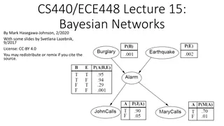
1. School of Computing Science Simon Fraser University Vancouver, Canada Relational Bayes Net Classifiers

2. Predicting Ground Facts Many relational models aim to predict specific facts Will the Raptors win the NBA final? Is Spectre likely to do well at the box office? Predictions for test instances The problem: relational data feature multiple instantiations of the same pattern 1,000 men give Spectre a high rating, 1,200 women give Spectre a high rating Bacchus, F.; Grove, A. J.; Koller, D. & Halpern, J. Y. (1992), From Statistics to Beliefs, in 'AAAI', pp. 602-608. Halpern, J. Y. (2006), From statistical knowledge bases to degrees of belief: an overview, in 'PODS', ACM, , pp. 110 113. 2

3. Frequencies and Individual Cases Statistical thinking derives conclusions about individual cases from properties of categories and ensembles Daniel Kahneman, Thinking Fast and Slow Probability learning instantiate predict values for individual cases Frequency Model inference 3 Learning Bayesian Networks for Complex Relational Data

4. Two Kinds of Relational Probabilities Relational Probability instantiate (?) P(first-order formulas) P(ground formulas) Degree of Belief type 2 probability Instance-level probability Relational Frequency Statistics type 1 probability Class-level probability inference (?) The Halpern instantiation principle: P( (X)) = P( (c)) where is a formula with free logical variable X, and c is a constant instantiating X Halpern, J. Y. (1990), 'An analysis of first-order logics of probability', Artificial Intelligence 46(3), 311--350. Bacchus, F. (1990), Representing and Reasoning with Probabilistic Knowledge: A Logical Approach to Probabilities, MIT Press. 4

5. Instantiation Principle for IID data First-Order P( (X)) 90% of birds fly P(Flies(B)) = 90% 0% of planes have crashed because of turbulence Ground Instance P( (c)) The probability that Tweety flies is 90% P(Flies(tweety)) = 90% The probability that Flight 3202 to Toronto crashes because of turbulence is 0% P(Turbulence_Crash(3202)) = 0% P(LivesNearBorder(oliver)) = 80% P(Turbulence_Crash(Plane)) = 0% P(LivesNearBorder(Canadian)) = 80% P( (X)) = P( (c)) 5 Learning Bayesian Networks for Complex Relational Data

6. The Instantiation Principle is valid but insufficient for relational data Example Goal: Predict gender of a specific user, Sam, from ratings. Data: Sam has rated 50 action movies. Sam has not rated 450 action movies. Frequencies: Suppose we know that P(gender(User)=M|HasRated(User,ActionMovie)=T)=58% P(gender(User)=M|HasRated(User,ActionMovie)=F)=50% This does not determine a unique value for P(gender(sam)=M). The insufficiency of the instantiation principle is one of the most consequential differences between relational and IID data. 6 Learning Bayesian Networks for Complex Relational Data

7. Multiple Instantiations Graph Instantiating a FOB with constants ground Bayes net or inference graph. HasRated(User,ActionMovie) gender(User) HR(sam,movie50) HR(sam,Spectre) HR(sam,DieHard) ... gender(sam) HR(sam,Scarface) HR(sam,Gladiator) HR(sam,movie500) ... 7 Neville, J. & Jensen, D. (2007), 'Relational Dependency Networks', Journal of Machine Learning Research 8, 653 692.

8. Many Models for Multiple Instantiations Parametrized Bayes Nets Probabilistic Relational Models, Markov Logic Networks, Bayes Logic Programs, Logical Bayesian Networks, Relational Probability Statistical-Relational Models (Lise Getoor, Taskar, Koller 2001) Model for Frequencies Class-Level Probabilities Model for Single Event Probabilities Instance-Level Probabilities Getoor, L. (2001), 'Learning Statistical Models From Relational Data', PhD thesis, Department of Computer Science, Stanford University. Getoor, L.; Taskar, B. & Koller, D. (2001), 'Selectivity estimation using probabilistic models', ACM SIGMOD Record 30(2), 461 472. 8

9. This Tutorial: Unified Approach Statistical thinking derives conclusions about individual cases from properties of categories and ensembles Daniel Kahneman, Thinking Fast and Slow Learning Bayesian Network statistical-relational model Frequencies Class-Level Single Event Probabilities Instance-Level instantiate new log-linear model 9

10. Bayesian Network Relational Classifier Log-linear classification model Learning Bayesian Networks for Complex Relational Data

11. Bayesian Network Relational Classification Classification problem: Define P(Y*=y|X*=x) for ground term Y* given values for all other ground terms X* Strictly easier than defining joint probability P(Y*=y,X*=x) Y* is the target node Instance-level probabilities are often modeled by viewing a first-order Bayesian network as a template (plate) model Instantiating a template model defines a ground Bayes net or inference graph The instantiated graph inherits parameters from class-level BN parameters for individuals from the same class are tied Kimmig, A.; Mihalkova, L. & Getoor, L. (2014), 'Lifted graphical models: a survey', Machine Learning, 1--45. Neville, J. & Jensen, D. (2007), 'Relational Dependency Networks', Journal of Machine Learning Research 8, 653 692. 11

12. Running Example We consider a simple example where the target node is the child node and has no children itself Let s introduce action movies as a new class of Movies called ActionMovies The problem is to predict the gender of Sam given that 1. Sam has rated 50 action movies 2. Sam has not rated 450 action movies 12 Learning Bayesian Networks for Complex Relational Data

13. Example Template Model P(HasRated(User,ActionMovie) = T) = 6% HasRated(User,ActionMovie) gender(User) P(gender(User)=M|HasRated(User,ActionMovie)=T)=58% P(gender(User)=M|HasRated(User,ActionMovie)=F)=50% Frequency Interpretation: Men are more likely to rate action movies than women are. 13 Learning Bayesian Networks for Complex Relational Data

14. Example Ground Model HR(sam,movie50) HR(sam,Spectre) HR(sam,DieHard) ... gender(sam) HR(sam,Scarface) HR(sam,Gladiator) HR(sam,movie500) ... Instantiations for users other than sam are not relevant and therefore not included 14 Neville, J. & Jensen, D. (2007), 'Relational Dependency Networks', Journal of Machine Learning Research 8, 653 692.

15. Combining Rules Multiple parent instances multiple conditional probabilities A method for combining the conditional probabilities is called a combining rule Multiplicative combining rule log-linear model (more below) 15 Learning Bayesian Networks for Complex Relational Data

16. Log-linear Bayesian Network Classification Formula Generalizes IID data classification formula Learning Bayesian Networks for Complex Relational Data

17. Classification and Random Selection Basic idea: score labels by comparing random selection likelihood for possible world (Y*=0,X*=x) to random selection likelihood for possible world (Y*=1,X*=x). (cf. Kimmig et al. 2014 Eq.4) It can be shown that random selection likelihood comparison combining rule = geometric mean 17 Learning Bayesian Networks for Complex Relational Data

18. General Classification Formula for Relational Data To compute P(target node = value| values for all other ground nodes), multiply: the geometric mean of P(target node = value|parent instance values) over all instances of parents for each child j of node, the geometric mean of P(childj=value|parent instance values, target node =value) over all instances of not-target parents of childj Normalize product of means for each possible target node value. Generalizes Markov blanket classification formula for i.i.d. data. Can be adjusted to consider relevant features only. 1. 2. 18 Learning Bayesian Networks for Complex Relational Data

19. Examples We illustrate the classification formula for two simplifying cases. 1. The target node has parents but no children. 2. The target node has children but not parents. The general classification formula combines both cases See auxiliary material for an example calculation with both parents and children. 19 Learning Bayesian Networks for Complex Relational Data

20. Example 1 Target Node has parents but no children Learning Bayesian Networks for Complex Relational Data

21. Example Template Model P(HasRated(User,ActionMovie) = T) = 6% HasRated(User,ActionMovie) gender(User) P(gender(User)=M|HasRated(User,ActionMovie)=T)=58% P(gender(User)=M|HasRated(User,ActionMovie)=F)=50% Frequency Interpretation: Men are more likely to rate action movies than women are. 21 Learning Bayesian Networks for Complex Relational Data

22. Calculation for gender(sam)=M P(gender(sam)= M) ((58%)50 (50%)450)1/500 0.507 T T T HR(sam,movie50) HR(sam,Spectre) HR(sam,DieHard) ... CP = 58% CP = 58% CP = 58% gender(sam) M CP = 50% CP = 50% CP = 50% F F F HR(sam,Scarface) HR(sam,Gladiator) HR(sam,movie500) ... 22 Learning Bayesian Networks for Complex Relational Data

23. Calculation for gender(sam)=W P(gender(sam)=W) ((42%)50(50%)450)1/500 0.491 T T T HR(sam,movie50) HR(sam,Spectre) HR(sam,DieHard) ... CP = 42% CP = 42% CP = 42% gender(sam) W CP = 50% CP = 50% CP = 50% F F F HR(sam,Scarface) HR(sam,Gladiator) HR(sam,movie500) ... 23 Learning Bayesian Networks for Complex Relational Data

24. Normalization Possible Value Score Probability M 0.507 0.508 W 0.491 0.492 So Sam is slightly more likely to be a man (50.8%) (because Sam has rated a fair number of action movies) The difference is small because most movies are unrated and therefore irrelevant 24 Learning Bayesian Networks for Complex Relational Data

25. Classification With Relevant Groundings Only Learning Bayesian Networks for Complex Relational Data

26. Eliminating Irrelevant Features In the example, unrated movies are irrelevant to the user of a gender: P(gender(User)=M|HasRated(User,ActionMovie)=F) = 50%, which is is also the prior probability P(gender=M). Most of the weight is on the irrelevant condition. In the example 450/500 instances are irrelevant. Relational models often consider only instantiations of relevant conditions. (Ngo and Haddaway, Heckerman et al.) Ngo, L. & Haddawy, P. (1997), 'Answering Queries from Context-Sensitive Probabilistic Knowledge Bases', Theoretical Computer Science 171(1-2), 147-177. D.Heckerman, C. M. & Koller, D. (2004), 'Probabilistic models for relational data', Technical report, Microsoft Research. 26

27. Calculation With gender(sam)=M for Relevant Features Only P(gender(sam)=M) (58%)50)1/50=58% T T T HR(sam,movie50) HR(sam,Spectre) HR(sam,DieHard) ... CP = 58% CP = 58% CP = 58% gender(sam) M In this simple case there is only one relevant parent value 27 Learning Bayesian Networks for Complex Relational Data

28. Calculation for gender(sam)=W for Relevant Features Only P(gender(sam)=W) ((42%)50)1/50=42% T T T HR(sam,movie50) HR(sam,Spectre) HR(sam,DieHard) ... CP = 42% CP = 42% CP = 42% gender(sam) W CP = 50% CP = 50% CP = 50% F F F HR(sam,Scarface) HR(sam,Gladiator) HR(sam,movie500) ... Eliminating irrelevant parent conditions increases the confidence that Sam is male (58% vs. 50.7%). 28 Learning Bayesian Networks for Complex Relational Data

29. Example 2 Target Node has children but no parents Learning Bayesian Networks for Complex Relational Data

30. Example Template Model P(HasRated(sam,ActionMovie)=T|gender(sam)=M)=7% P(HasRated(sam,ActionMovie)=T|gender(sam)=W)=5% HasRated(User,ActionMovie) gender(User) P(gender(User)=M)=50% Frequency Interpretation: Men are more likely to rate action movies than women are. 30 Learning Bayesian Networks for Complex Relational Data

31. Calculation for gender(sam)=M P(gender(sam)= M) ((7%)50 (93%)450)1/500 50% 0.452 T HR(sam,DieHard) T T HR(sam,movie50) HR(sam,Spectre) ... CP = 7% CP = 7% CP = 7% gender(sam) CP = 50% M CP = 93% CP = 93% CP = 93% F F F HR(sam,Scarface) HR(sam,Gladiator) HR(sam,movie500) ... 31 Learning Bayesian Networks for Complex Relational Data

32. Calculation for gender(sam)=W P(gender(sam)= M) ((5%)50 (95%)450)1/500 50% 0.445 T HR(sam,DieHard) T T HR(sam,movie50) HR(sam,Spectre) ... CP = 5% CP = 5% CP = 5% gender(sam) CP = 50% W CP = 95% CP = 95% CP = 95% F F F HR(sam,Scarface) HR(sam,Gladiator) HR(sam,movie500) ... 32 Learning Bayesian Networks for Complex Relational Data

33. Normalization Possible Value Score Probability M 0.452 0.503 W 0.445 0.496 So Sam is slightly more likely to be a man (50.3%) (because Sam has rated a fair number of action movies) The difference is small because most movies are unrated and therefore irrelevant 33 Learning Bayesian Networks for Complex Relational Data

34. Log-linear Relational Models Learning Bayesian Networks for Complex Relational Data

35. Log-linear Relational Models Log-linear model: weighted sum of factors/feature functions/sufficient statistics P(Y*= y| X-Y i *= x) exp{ wi fi(y,x) } output label of ground target node In our Bayes net classification formula: feature = (relevant) parent-child value combination feature function = proportion of parent-child value instantiations weight = log(conditional probability) BN structure learning = discovery of conjunctive features input labels for other ground nodes real-valued function associated with feature i Kimmig, A.; Mihalkova, L. & Getoor, L. (2014), 'Lifted graphical models: a survey', Machine Learning, 1--45. 35

36. More on Log-linear Relational Models Very common model class for both discriminative and generative learning, e.g. Random Selection Likelihood. Markov Logic Network. Relational Logistic Regression (Kazemi et al. 2014). Highly expressive: can represent other relational aggregation rules (Kazemi et al. 2014). Kazemi, S. M.; Buchman, D.; Kersting, K.; Natarajan, S. & Poole, D. (2014), Relational Logistic Regression, in 'Principles of Knowledge Representation and Reasoning:, KR 2014. Kimmig, A.; Mihalkova, L. & Getoor, L. (2014), 'Lifted graphical models: a survey', Machine Learning, 1--45. 36

37. Discovering Features for Classification Learning Bayesian Networks for Complex Relational Data

38. Visualization Learned features can be visualized in a data matrix Row = target instance Column = conjunctive feature = child-parent value assignment Cell entry = instantiation proportion/count of feature for target instance We provide a tool for producing this data matrix automatically given a target functor 38

39. Data Matrix For Classification gender(sam) HasRated(sam,ActionMovie) ln(0.58/0.42)=0.32 ln(0.5/0.5)=0 UserID gender(U) HasRated(U,AM) =T HasRated(U,AM)=F sam jill .... ? W 0.1 0.2 0.9 0.8 Our BN classification formula is a logistic regression model for these features. Weights = ln(conditional probability ratios for different output labels). 39 Learning Bayesian Networks for Complex Relational Data

40. Propositionalization The data matrix can be treated as a pseudo-i.i.d. view (Lippi et al., Lavrac et al.) provide as input to classification learners for i.i.d. data Converting relational data to features for i.i.d. learning is called propositionalization A form of Extract, Transform, Load Features in a pseudo i.i.d. data view are often computed using aggregate functions (e.g. average, mode) See anomaly supplement for movie world example Lippi, M.; Jaeger, M.; Frasconi, P. & Passerini, A. (2011), 'Relational information gain', Machine Learning 83(2), 219--239. Lavrac, N.; Perovsek, M. & Vavpetic, A. (2014), Propositionalization Online'ECML', Springer, , pp. 456 459. 40

41. Dependency Networks Learning Bayesian Networks for Complex Relational Data

42. Dependency Networks AKA Markov blanket networks Increasingly popular for relational data. Defined by a local conditional distribution for each random variable Y*: P(Y*=y|X*=x) Allows collective inference via Gibbs sampling We just showed Bayesian network dependency network Can compare with other dependency network learning Hofmann, R. & Tresp, V. (1998), Nonlinear Markov networks for continuous variables, in 'Advances in Neural Information Processing Systems', pp. 521--527. Heckerman, D.; Chickering, D. M.; Meek, C.; Roundthwaite, R.; Kadie, C. & Kaelbling, P. (2000), 'Dependency Networks for Inference, Collaborative Filtering, and Data Visualization', JMLR 1, 49 75. Neville, J. & Jensen, D. (2007), 'Relational Dependency Networks', Journal of Machine Learning Research 8, 653--692. 42

43. Accuracy Comparison RDN_Boost MLN_Boost RDN_Bayes 1.20 1.00 0.80 PR 0.60 0.40 0.20 0.00 UW Mondial Hepatitis Muta MovieLens(0.1M) 0.00 -0.10 -0.20 -0.30 CLL -0.40 -0.50 -0.60 -0.70 Leave-one-out over all unary functors PR = area under precision-recall curve CLL: conditional log-likelihood 43

44. Learning Time Comparison (recall) Dataset # Predicates # tuples RDN_Boost MLN_Boost RDN_Bayes 14 18 19 11 7 7 1,010,051 UW Mondial Hepatitis Mutagenesis MovieLens(0.1M) MovieLens(1M) 612 870 15 0.3 27 0.9 251 5.3 118 6.3 44 4.5 min 31 1.87 min >24 hours 19 0.7 42 1.0 230 2.0 49 1.3 1 0.0 102 6.9 286 2.9 1 0.0 1 0.0 10 0.1 11,316 24,326 83,402 >24 hours Standard deviations are shown Units are seconds unless otherwise stated Natarajan, S.; Khot, T.; Kersting, K.; Gutmann, B. & Shavlik, J. W. (2012), 'Gradient-based boosting for statistical relational learning: The relational dependency network case', Machine Learning 86(1), 25-56. Schulte, O.; Qian, Z.; Kirkpatrick, A. E.; Yin, X. & Sun, Y. (2016), 'Fast learning of relational dependency networks', Machine Learning, 1 30. 44

45. RDN-Bayes uses more relevant predicates and more first-order variables Our best predicate for each database: # extra predicate s 11 6 4 4 5 1 # extra first order variables 1 2 1 2 1 1 Target Predicate religion gender student sex ind1 gender Database Mondial IMDB UW-CSE Hepatitis Mutagenesis MovieLens CLL-diff 0.58 0.30 0.50 0.20 0.56 0.26 45 Learning Bayesian Networks for Complex Relational Data

46. Summary: Log-linear Models With Proportions Defines a relational classification formula for First-order Bayesian Networks. Generalizes the iid classification formula. proportions are on the same scale [0,1] unlike counts; addresses ill-conditioning (Lowd and Domingos 2007) Also effective for dependency networks with hybrid data types (Ravkic et al. 2015) Random selection semantics provides a theoretical foundation Lowd, D. & Domingos, P. (2007), Efficient Weight Learning for Markov Logic Networks, in 'PKDD', pp. 200 211. Ravkic, I.; Ramon, J. & Davis, J. (2015), 'Learning relational dependency networks in hybrid domains', Machine Learning 46