Utilizing Pandas for Efficient Data Handling

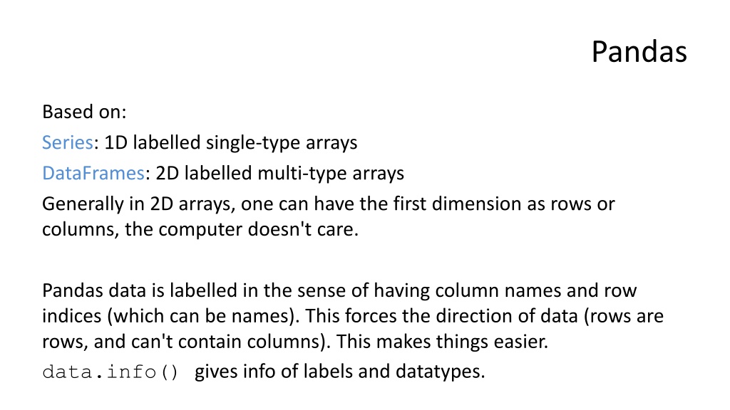
Pandas Based on: Series: 1D labelled single-type arrays DataFrames: 2D labelled multi-type arrays Generally in 2D arrays, one can have the first dimension as rows or columns, the computer doesn't care. Pandas data is labelled in the sense of having column names and row indices (which can be names). This forces the direction of data (rows are rows, and can't contain columns). This makes things easier. data.info() gives info of labels and datatypes.

Creating Series # nan == Not a Number data = [1,2,3,numpy.nan,5,6] unindexed = pandas.Series(data) indices = ['a', 'b', 'c', 'd', 'e'] indexed = pandas.Series(data, index=indices) data_dict = {'a' : 1, 'b' : 2, 'c' : 3} indexed = pandas.Series(data_dict) fives = pandas.Series(5, indices) # Fill with 5s. named = pandas.Series(data, name='mydata') named.rename('my_data') print(named.name)

Datetime data Treated specially date_indices = pandas.date_range('20130101', periods=6, freq='D') Generates six days, '2013-01-01' to '2013-01-06'. Although dates have hyphens when printed, they should be used without for indexing etc. Frequency is days by default, but can be 'Y', 'M', 'W' or 'H', 'min', 'S', 'ms', 'um', 'N' and others: http://pandas.pydata.org/pandas-docs/stable/timeseries.html#offset-aliases

Print As with numpy. Also: df.head() df.tail(5) df.index df.columns df.values df.sort_index(axis=1, ascending=False) df.sort_values(by='col1') First few lines Last 5 lines

Indexing named[0] named[:0] named[[0,1]] 1 a 1 a 1 b 2 1 named["a"] "a" in named == True Returns default if index not found named.get('f', numpy.nan) Can also take equations: a[a > a.median()]

Looping for value in series: etc. But generally unneeded: most operations take in series and process them elementwise.

DataFrames Dict of 1D ndarrays, lists, dicts, or Series 2-D numpy.ndarray Series data_dict = {'col1' : [1, 2, 3, 4], 'col2' : [10, 20, 30, 40]} Lists here could be ndarrays or Series. indices = ['a', 'b', 'c', 'd'] df = pandas.DataFrame(data_dict, index = indices) If no indices are passed in, numbered from zero. If data shorter than current columns, filled with numpy.nan.

a = pandas.DataFrame.from_items( [('col1', [1, 2, 3]), ('col2', [4, 5, 6])]) col1 col2 1 2 3 0 1 2 4 5 6 a = pandas.DataFrame.from_items( [('A', [1, 2, 3]), ('B', [4, 5, 6])], orient='index', columns=['col1', 'col2', 'col3']) col1 col2 col3 A 1 2 3 B 4 5 6

I/O df = pandas.read_csv('data.csv') df.to_csv('data.csv') df = pandas.read_excel( 'data.xlsx', 'Sheet1', index_col=None, na_values=['NA']) df.to_excel('data.xlsx', sheet_name='Sheet1') df = pandas.read_json('data.json') json = df.to_json() Can then be written to a text file. Wide variety of other formats including HTML and the local CTRL-C copy clipboard: http://pandas.pydata.org/pandas-docs/stable/io.html

Adding to DataFrames concat() join() append() insert() inserts columns at a specific location adds dataframes joins SQL style adds rows Remove df.sub(df['col1'], axis=0) (though you might also see df - df['col1'])

Broadcasting When working with a single series and a dataframe, the series will sometimes be assumed a row. Check. This doesn't happen with time series data. More details on broadcasting, see: http://pandas.pydata.org/pandas- docs/stable/dsintro.html#data-alignment-and-arithmetic

Indexing By name: (you may also see at() used) named.loc['row1',['col1','col2']] Note that with slicing on labels, both start and end returned. Note also, not function. iloc[1,1] used for positions.

Indexing Operation Syntax Result Select column df[col] Series Select row by label df.loc[label] Series representing row Select row by integer location df.iloc[loc] Series representing row Slice rows df[5:10] DataFrame Select rows by boolean 1D array df[bool_array] DataFrame Pull out specific rows df.query('Col1 < 10') (See also isin() )

Sparse data df1.dropna(how='any') df1.fillna(value=5) a = pd.isna(df1) Drop rows associated with numpy.nan Boolean mask array

Stack df.stack() Combines the last two columns into one with a column of labels: A B 10 20 30 40 A B A B unstack() does the opposite. For more sophistication, see pivot tables: http://pandas.pydata.org/pandas-docs/stable/reshaping.html#pivot-tables 10 20 30 40

Looping for col in df.columns: series = df[col] for index in df.indices: print(series[index]) But, again, generally unneeded: most operations take in series and process them elementwise. If column names are sound variable names, they can be accessed like: df.col1

Columns as results df['col3'] = df['col1'] + df['col2'] df['col2'] = df['col1'] < 10 # Boolean values df['col1'] = 10 df2 = df.assign(col3 = someFuntion + df['col1'], col4 = 10) Assign always returns a copy. Note names not strings. Cols inserted alphabetically, and you can't use cols created elsewhere in the statement.

Functions Generally functions on two series result in the union of the labels. Generally both series and dataframes work well with numpy functions. Note that the documentation sometimes calls functions "operations". Operations generally exclude nan. df.mean() Per column df.mean(1) Per row Complete API of functions at: http://pandas.pydata.org/pandas-docs/stable/api.html

Useful operations df.describe() df.apply(function) df.value_counts() df.T or pandas.transpose(df) Quick stats summary Applies function,lambda etc. to data in cols Histogram Transpose rows for columns.

Categorical data Categorical data can be: renamed sorted grouped by (histogram-like) merged and unioned http://pandas.pydata.org/pandas-docs/stable/categorical.html

Time series data Time series data can be: resampled at lesser frequencies converted between time zones and representations sub-sampled and used in maths and indexing analysed for holidays and business days shifted/lagged http://pandas.pydata.org/pandas-docs/stable/timeseries.html

matlibplot wrapped in pandas: Complex plots may need matplotlib.pyplot.figure() calling first. Plotting series.plot() Line plot a series Line plot a set of series Plot data against another dataframe.plot() dataframe.plot(x='col1', y='col2') bar or barh hist box kde or density area scatter hexbin pie http://pandas.pydata.org/pandas-docs/stable/visualization.html bar plots histogram boxplot density plots area plots scatter plots hexagonal bin plots pie graphs

Packages built on pandas Statsmodels sklearn-pandas Bokeh seaborn yhat/ggplot Plotly IPython/Spyder GeoPandas http://pandas.pydata.org/pandas-docs/stable/ecosystem.html Statistics and econometrics Scikit-learn (machine learning) with pandas Big data visualisation Data visualisation Grammar of Graphics visualisation Web visualisation using D3.js Both allow integration of pandas dataframes Pandas for mapping