Understanding Solvency II for Insurers and Reinsurers

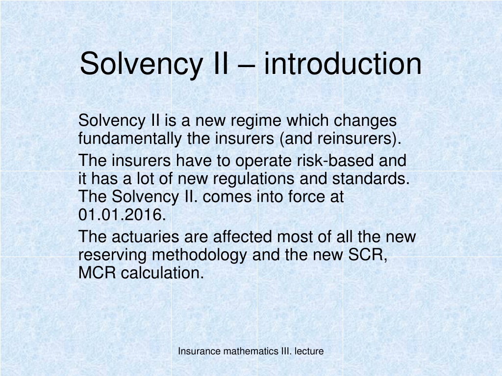
Solvency II introduction Solvency II is a new regime which changes fundamentally the insurers (and reinsurers). The insurers have to operate risk-based and it has a lot of new regulations and standards. The Solvency II. comes into force at 01.01.2016. The actuaries are affected most of all the new reserving methodology and the new SCR, MCR calculation. Insurance mathematics III. lecture

Solvency II. New SCR calculation SCR A dj OP BSCR Market Health Default Non-life Lif e Intang Premium reserve Interest rate SLT Health Non-SLT Health CAT Revision Premium reserve Equity Mortality Lapse Mortality Property Longev ity Longevity Lapse CAT Disabili morbidi ty ty Disability morbidity Spread Currency Lapse Lapse Concentration Expenses Expenses CAT Revision Insurance mathematics III. lecture

Solvency II. Reserving I. Reserving methodology is based on the best estimate assumptions plus additional risk margin. The best estimate shall correspond to the probability- weighted average of future cash-flows within the contract boundary, taking account of the time value of money (expected present value of future cash-flows), using the relevant risk-free interest rate term structure. Insurance mathematics III. lecture

Solvency II. Reserving II. The risk margin shall be such as to ensure that the value of the technical provisions is equivalent to the amount that insurance and reinsurance undertakings would be expected to require in order to take over and meet the insurance and reinsurance obligations. boundary: contract shall be taking into Contract consideration till the date when one of partners (insurer or insured) can quit from policy without any consequence. In non-life section the typical possibility to exiting from policy is 1 year, it means that usually we have to calculate premium till end of first policy year but claims according to first policy year can be reported later. Insurance mathematics III. lecture

Solvency II. Reserving III. In non-life section we can calculate separately reserve for premium and claims. The ultimate reserve will be the sum of reserve for premium and reserve for claims. The reserve for premium can be calculated with the next formula: ??????? =??? 1 ?????? ????? ??? ???? ????? 1 + ????????_???? Remark: if the product is profitable then the amount has negative sign. Insurance mathematics III. lecture

Solvency II. Reserving IV. where UPR signs the Unearned Premium Reserve; PbCanc signs the probability of cancellation; ClPay signs the claim payment for claims which occurred before policy anniversary; DAC signs the deferred acquisition costs; ClHC signs the claims handling costs for claims which occurred before policy anniversary; MainC signs the maintenance cost which are affected till policy anniversary. Insurance mathematics III. lecture

Solvency II. Reserving V. Example: Let the total portfolio is one policy with the next data: Beginning date: Annual premium: Probability of cancellation: Expected loss ratio: Commission: Claims handling costs: Maintenance costs: Discount rate: 01.10.2021 50.000 Ft 15% yearly 70% 6% 9% of claim 10% of premium 5% Insurance mathematics III. lecture

Solvency II. Reserving VI. Example (continued) We are calculating the reserve for premium at 31.12.2021. 9 9 ?????? = 12 15% = 11,25% ??? = 12 50000 = 37500 ??? 1 ?????? = 37500 88,75% = 33281 ????? = ???? ????????? = 33281 70% = 23297 ??? = ???? ????????????? = 37500 6% = 2250 ???? = ????? ?????????????? = 23297 9% = 2097 ????? = ???? ?????????????? = 37500 10% = 3750 Insurance mathematics III. lecture

Solvency II. Reserving VII. Example (continued) ????? ??????????? = 33281 23297 2250 2097 3750 = 1887 ??????? =????? ??????????? 1 + ????????_???? =1887 1,05= 1797 Reserve for claims Actuaries have to estimate reported and not yet reported claims together plus claims handling cost in the future. It shall be applied the discount rate according to year of expected claim payment. If there is no differing information (e.g. changing of portfolio) we can use previous information for claims. Insurance mathematics III. lecture

Solvency II. Reserving VIII. One possible method is as follows: OS reserve 1.step: Calculating the ratio of previous payments related to lagging time (year, quarter year, month). 2.step: Calculating the ratio of actual OS reserve according to occurring date (year, quarter year, month). 3.step: Calculating the real OS need based on result of earlier OS reserve (e.g. result is +10% ,then the real OS need is lower with 10%). 4.step: Estimating the payment of real OS need based on 1. and 2. step. 5.step: Discounting the result of 4. step with adequate discount factors. Insurance mathematics III. lecture

Solvency II. Reserving IX. Example: We have 126.000.000 Ft OS reserve (according to Solvency I.) and we have to calculate Best Estimate. 1. step: we have data from past payments according to lagging as follows: 0. year 60% 1.year 30% 2.year 9% 3.year 1% 2. step: we have data about OS reserve occurring date as follows: 2018 2019 1.000.000 5.000.000 2020 2021 20.000.000 100.000.000 Insurance mathematics III. lecture

Solvency II. Reserving X. 3. step: Result of earlier OS reserve is +5%. It means the real OS need is as follows: 2018 2019 2020 2021 20000000 100000000 1000000 1,05 5000000 =19047618 =95238090 =4761905 = 952381 1,05 1,05 1,05 4. step: Payment estimation as follows according to earlier steps: Insurance mathematics III. lecture

Solvency II. Reserving XI. Occurring/ Paying year 2022 2023 2024 2018 952381 2019 4761905 2020 9 1 19047618 19047618 10 10 9 40 2021 95238090 30 1 95238090 95238090 40 40 Total 94.285.620 23.333.332 2.380.952 Insurance mathematics III. lecture

Solvency II. Reserving XII. 5. step: The discount rates are given as follows: 1. year 5% 2. year 4% 3. year 3% Then the reserve for OS reserve will be the next: ????? =94285620 +23333332 1,05 1,04+ 2380952 1,05 1,04 1,03= 113.280.621 1,05 Insurance mathematics III. lecture

Solvency II. Reserving XIII. IBNR It can be calculated with classical methods (just one difference: we have to take into consideration the result of earlier IBNR) it shall be considered which part of IBNR when will be paid (according to estimation). At the end the discount factors shall be applied. Insurance mathematics III. lecture

Solvency II. Reserving XIV. Example: 0 1 2 3 2018 50000 55000 57000 57500 Cumulated, lagging triangle 2019 65000 70000 72000 2020 75000 85000 85000 2021 Insurance mathematics III. lecture

Solvency II. Reserving XV. Example (continued): We are using chain-ladder method, we suppose that the triangle is complete. 0 1 2 3 2018 50000 55000 57000 57500 Year IBNR 2018 2019 2020 2021 Total 0 2019 65000 70000 72000 72632 632 2020 75000 85000 87720 88489 3.489 12.804 16.925 2021 85000 93947 96954 97804 Insurance mathematics III. lecture

Solvency II. Reserving XVI. Example (continued): Occurring/ Paying year 2022 2023 2024 2018 0 2019 632 2020 2720 769 2021 8947 3006 850 Total 12.299 3.775 850 Insurance mathematics III. lecture

Solvency II. Reserving XVII. The discount rates are given as follows: 1. year 5% 2. year 4% 3. year 3% Then the reserve for IBNR claims will be the next: ??????? =12299 3775 850 + 1,05 1,04+ 1,05 1,04 1,03= 15927 1,05 Insurance mathematics III. lecture

Solvency II. Difficulties I. There are a lot of questions, difficulties related to Solvency II., because this is a total new specifications - which have to be applied - are not exactly clear in each case. I highlight just two points from these questions regime and the technical 1. Segmentation In Solvency II. the target is making homogenous risk portfolio and for these groups using the specifications. In the other side (in non- life section) there is given the business lines which have to be applied. These two requirements would be controversy if one homogenous risk portfolio does not fit to the given business lines. Insurance mathematics III. lecture

Solvency II. Difficulties II. 2. Claim inflation There is not clear whether there is possible to consider claim inflation or not. And if the answer is yes then how should be calculated. (In EU there are countries in which has high inflation but other countries have no high inflation.) Insurance mathematics III. lecture