Understanding Longitudinal Particle Motion in Accelerators
Explore the concepts of longitudinal motion in particle accelerators, including acceleration in periodic structures, slip factors, phase stability, longitudinal acceleration, and phase stability analysis. Dive into the intricate details of synchrotron motion and synchrotron tune to enhance your understanding of particle dynamics in accelerators.

Download Presentation

Please find below an Image/Link to download the presentation.
The content on the website is provided AS IS for your information and personal use only. It may not be sold, licensed, or shared on other websites without obtaining consent from the author. If you encounter any issues during the download, it is possible that the publisher has removed the file from their server.
You are allowed to download the files provided on this website for personal or commercial use, subject to the condition that they are used lawfully. All files are the property of their respective owners.
The content on the website is provided AS IS for your information and personal use only. It may not be sold, licensed, or shared on other websites without obtaining consent from the author.
E N D
Presentation Transcript
Longitudinal Motion 1 Eric Prebys, FNAL
Acceleration in Periodic Structures We consider motion of particles either through a linear structure or in a circular ring Always negative 1 p p = 2 p p In both cases, we can adjust the RF phases such that a particle of nominal energy arrives at the the same point in the cycle s E Goes from negative to positive at transition 1 1 p p = 2 2 p p t Lecture 8 - Longitudinal Motion 1 USPAS, Knoxville, TN, Jan. 20-31, 2014 2
Slip Factors and Phase Stability The sign of the slip factor determines the stable region on the RF curve. >0 (above transition) <0 (linacs and below transition) (t ) (t ) V V bunch Particles with lower E arrive earlier and see greater V. Particles with lower E arrive later and see greater V. t t Nominal Energy Nominal Energy Lecture 8 - Longitudinal Motion 1 USPAS, Knoxville, TN, Jan. 20-31, 2014 3
Longitudinal Acceleration Consider a particle circulating around a ring, which passes through a resonant accelerating structure each turn Harmonic number (integer) h ( ) = + = 2 sin ; V V t E 0 0 Period of nominal energy particle The energy gain that a particle of the nominal energy experiences each turn is given by eV E E sin 0 1 + = + Synchronous phase n n s Where the this phase will be the same for a particle on each turn A particle with a different energy will have a different phase, which will evolve each turn as p rf n n = + = + 1 1 p E rf + E = use n 2 p E 2 p E S Lecture 8 - Longitudinal Motion 1 USPAS, Knoxville, TN, Jan. 20-31, 2014 4
Phase Stability Thus the change in energy for this particle for this particle will evolve as ( n n eV E E sin 0 1 + = + d ) sin n s So we can write rf = E 2 dn E S d E ( ) = sin sin eV 0 n s dn 0 eV 2 2 d ( ) rf = sin sin n s 2 dn E S d Multiply both sides by and integrate over dn dn d2j dn2 dj dndn =eV0wrfth = -eV0wrfth ESb2 )dj dndn ( sinj(n)-sinjs ESb2 2 dj dn 1 2 ( )+constant cosj +jsinjs 2+2eV0ESb2 wrfth ( ) = constant ( ) DE cosj +jsinjs Lecture 8 - Longitudinal Motion 1 USPAS, Knoxville, TN, Jan. 20-31, 2014 5
Synchrotron motion and Synchrotron Tune Going back to our original equation + dn eV 2 d ( ) 0 rf = sin sin 0 n s 2 2 E S For small oscillations, sin ( ) = sin cos cos n s s n s s And we have E rf eV 2 d 0 + = cos 0 s 2 2 dn S This is the equation of a harmonic oscillator with 0 0 eV eV 1 rf rf = = cos cos n s s s 2 2 2 E E S S Angular frequency wrt turn (not time) synchrotron tune = number of oscillations per turn (usually <<1) Lecture 8 - Longitudinal Motion 1 USPAS, Knoxville, TN, Jan. 20-31, 2014 6
Longitudinal Emittance We want to write things in terms of time and energy. We have can write the longitudinal equations of motion as 1 = ( ) ( ) t n n rf ( ) 1 ( ) d t n d n = = ( ) E n 2 dn dn E rf S We can write our general equation of motion for out of time particles as ( dDt dn 1 )+ ( ) Dt(n)= Dt0cos 2pnsn sin 2pnsn 2pns 0 th ( )+ ( ) = Dt0cos 2pnsn DE0sin 2pnsn 2pESb2ns DE(n)=ESb2 dDt(n) dn th )-2pESb2ns ( ( ) = DE0cos 2pnsn Dt0sin 2pnsn th Lecture 8 - Longitudinal Motion 1 USPAS, Knoxville, TN, Jan. 20-31, 2014 7
So we can write th ( ) ( ) cos 2pnsn sin 2pnsn = Dt0 DE 2pESb2ns Dt(n) DE(n) -2pESb2ns th ( ) ( ) sin 2pnsn cos 2pnsn 0 We see that this is the same form as our equation for longitudinal motion with =0, so we immediately write ( ) ( ) t cos 2 sin 2 ( ) n n t n 0 s L s = ( ) ( ) E sin 2 cos 2 ( ) n n E n L s s 0 Where 0 eV 1 rf = cos s s 2 2 E S 1 = = ; = L L 2 0 2 2 cos E eV E S s rf S s L Lecture 8 - Longitudinal Motion 1 USPAS, Knoxville, TN, Jan. 20-31, 2014 8
E We can define an invariant of the motion as t Area= L units generally eV-s What about the behavior of t and E separately? Note that for linacs or well-below transition ( ) ( )4 1 1 1 = 3 2 3 2 ; E t 4 2 Lecture 8 - Longitudinal Motion 1 USPAS, Knoxville, TN, Jan. 20-31, 2014 9
Large Amplitude Oscillations We can express period of off-energy particles as dt = p = n E n 2 dn p E s ( ) d ( ) = sin sin E eV t 0 n rf n s dn d d dn dt So ( ) ( ) = E E d d dt d d d ( ) ( ) E E Use: d d = = dt d dt = 2 L 0 2 rf cos eV E dn dt dn rf S s 2 eV E = 0 sin sin s s E rf 1 = sin sin s 2 2 cos E rf s L Lecture 8 - Longitudinal Motion 1 USPAS, Knoxville, TN, Jan. 20-31, 2014 10
Continuing sin sin ( ) = s Ed E 2cos rf 2 L s Integrate ( 2 cos + + cos sin cos sin 1 ) 2 = 0 0 s s E 2 rf 2 L s The curve will cross the axis when E=0, which happens at two points defined by sin cos 1 1 + = + cos sin 0 0 s s Phase trajectories are possible up to a maximum value of 0. Consider . ); sin (cos 0 0 = + s s 1 . Limit is at maximum of 1.5 1 or = sin sin 0 0.5 , 0 max s 0 = 0 -6 -1 4 , 0 max s s -0.5 unbound , 0 -1 bound max -1.5 -2 Lecture 8 - Longitudinal Motion 1 USPAS, Knoxville, TN, Jan. 20-31, 2014 11
Longitudinal Separatrix The other bound of motion can be found by sin cos max , 1 max , 1 + = + + ( sin cos( ) ) sin s s s s = ( cos ) s s s The limiting boundary (separatrix) is defined by 2 sin cos 2 E cos ( ) + + cos sin ( ) = s s s s 2 rf 2 L s The maximum energy of the bucket can be found by setting = s + cos 2 cos 2 2 sin sin ( ) 2 = 2 s s s s E b 2 rf s L 2 1 tan s s = 2 E b rf L Lecture 8 - Longitudinal Motion 1 USPAS, Knoxville, TN, Jan. 20-31, 2014 12
Bucket Area The bucket area can be found by integrating over the area inside the separatrix (which I won t do) 16 A ( ) ( )= s = ; b f f s rf L Lecture 8 - Longitudinal Motion 1 USPAS, Knoxville, TN, Jan. 20-31, 2014 13
Transition Crossing T We learned that for a simple FODO lattice so electron machines are always above transition. Proton machines are often designed to accelerate through transition. ( ) ( ) ( ) 0 = 0 0 As we go through transition Recall At transition: eV 1 Dtmax constant DEmax 0 rf = cos s s 2 2 E S t = = max E L 2 cos eV E 0 max rf S s so these both go to zero at transition. To keep motion stable 2 cos below 0 transitio n; 0 s s 2 cos above 0 transitio n; s s Lecture 8 - Longitudinal Motion 1 USPAS, Knoxville, TN, Jan. 20-31, 2014 14
Effects at Transition As the beam goes through transition, the stable phase must change Problems at transition (pretty thorough treatment in S&E 2.2.3) Beam loss at high dispersion points Emittance growth due to non-linear effects Increased sensitivity to instablities Complicated RF manipulations near transition Much harder before digital electronics Lecture 8 - Longitudinal Motion 1 USPAS, Knoxville, TN, Jan. 20-31, 2014 15
Accelerating Structures The basic resonant structure is the pillbox = ) t ( , E E r z ) = ( , B B r t Maxwell s Equations Become: 1 1 1 E E ( ) = = z B rB 2 2 c t r r c t Boundary Conditions: B B E = = 0 E B = = z E || t r t Differentiating the first by t and the second by r: 1 rB r r t 2 1 r 1 c B B E ( ) = + = z 2 2 r t t t 2 B E = z 2 r r t 2 2 1 r 1 c E E E + = z z z 2 2 2 r r t Lecture 8 - Longitudinal Motion 1 USPAS, Knoxville, TN, Jan. 20-31, 2014 16
General solution of the form + = i t ( ) E E r e z Which gives us the equation 0thorder Bessel s Equation 2 1 z z + + = = 0 ( ) E E E E r E J r 0 0 z 2 r c c 0th order Bessel function First zero at J(2.405), so lowest mode c 2 0= . 2 405 f R 0 B E = = = i t i t ( ) z E J r e i B r e 0 r c c t 1 0 1 = = ( ) B r i E J r i E J r 0 0 1 c c c c Lecture 8 - Longitudinal Motion 1 USPAS, Knoxville, TN, Jan. 20-31, 2014 17
Transit Factor In the lowest pillbox mode, the field is uniform along the length (vp= ), so it will be changing with time as the particle is transiting, thus a very long pillbox would have no net acceleration at all. We calculate a transit factor Assume peak in middle / 2 L z v fL fL L cos 2 eE f dz sin eE sin 0 0 v energy gain sin u f v v = = = / 2 T fL eE L eE L eE L u 0 0 0 v Example: 5 MeV Protons (v~.1c) f=200MHz T=85% u~1 c = 57 = . 2 405 cm R 2 f v = = 9 . 4 cm L u f Sounds kind of short, but is that an issue? Lecture 8 - Longitudinal Motion 1 USPAS, Knoxville, TN, Jan. 20-31, 2014 18
Power dissipation in RF Cavities Volume=L R2 Energy stored in cavity R 1 1 1 1 2 1 f ( . 2 ) = + = = = 2 2 2 0 2 0 2 0 2 dr 2 405 U E B dV E dV LE rJ r VE J 0 0 max 0 0 1 2 2 2 2 c 0 0 =(.52)2~25% Power loss: Magnetic field at boundary Surface current density J [A/m] l d = = = B LB I LJ . 0 0 enclosed 1 = J B B 0 2 ends Cylinder surface Average power loss per unit area is 1 1 2 2 R = = 2 1 E p J B = RLJ + 2 2 0 c 2 2 2 P R J r rdr s s 2 0 2 1 1 s 2 c c 0 0 2 Average over cycle + 1 E R ( . 2 ) = 2 0 2 1 405 RL J 1 s 2 Z L 0 1 = = = (impedance 0 where 376 73 . of free space) Z c 0 0 c 0 0 Lecture 8 - Longitudinal Motion 1 USPAS, Knoxville, TN, Jan. 20-31, 2014 19
The figure of merit for cavities is the Q, where ( ( E 2 ) Stored Energy U = 2 Q ) Energy Lost per Cycle P 2 0 2 2 . 2 ( 405 ) R LJ = 0 1 + 1 E R 2 2 . 2 ( 405 ) Z RL J 0 1 Z 1 s = Z L c 0 0 0 2 0 2 0 Z R c = = . 2 405 0 0 + 1 + 1 R R 2 2 Z s s L L = 0 . 2 405 + 1 R 2 s L So Q not very good for short, fat cavities! Lecture 8 - Longitudinal Motion 1 USPAS, Knoxville, TN, Jan. 20-31, 2014 20
Drift Tube (Alvarez) Cavity Put conducting tubes in a larger pillbox, such that inside the tubes E=0 Bunch of pillboxes Drift tubes contain quadrupoles to keep beam focused Gap spacing changes as velocity increases v d = f Fermilab low energy linac Inside Lecture 8 - Longitudinal Motion 1 USPAS, Knoxville, TN, Jan. 20-31, 2014 21
Shunt Impedance If we think of a cavity as resistor in an electric circuit, then V V P = 2 2 V = R R P By analogy, we define the shunt impedance for a cavity as ( ) gain voltage P ( ) 2 2 E LT = 0 R s P 2 0 2 Z L T = We want Rs to be as large as possible + R R 2 1 . 2 ( 405 ) J s 1 L Lecture 8 - Longitudinal Motion 1 USPAS, Knoxville, TN, Jan. 20-31, 2014 22
Other Types of Accelerating Structures cavities E v d = Lecture 8 - Longitudinal Motion 1 USPAS, Knoxville, TN, Jan. 20-31, 2014 23
Sources of RF Power For frequencies above ~300 MHz, the most common power source is the klystron , which is actually a little accelerator itself Electrons are bunched and accelerated, then their kinetic energy is extracted as microwave power. Lecture 8 - Longitudinal Motion 1 USPAS, Knoxville, TN, Jan. 20-31, 2014 24
Sources of RF Power (contd) For lower frequencies (<300 MHz), the only sources significant power are triode tubes, which haven t changed much in decades. 53 MHz Power Amplifier for Booster RF cavity FNAL linac 200 MHz Power Amplifier Lecture 8 - Longitudinal Motion 1 USPAS, Knoxville, TN, Jan. 20-31, 2014 25


 Cavity")


")