Understanding Interpolation: Methods and Applications
Interpolation is a technique used to estimate values between known data points. This content covers the concept of interpolation, its applications in solving real-world problems like rocket velocity and specific heat calculations, and methods such as spline interpolation. Explore how interpolation helps in reading between the lines of data points to find missing values effectively.
Download Presentation

Please find below an Image/Link to download the presentation.
The content on the website is provided AS IS for your information and personal use only. It may not be sold, licensed, or shared on other websites without obtaining consent from the author. Download presentation by click this link. If you encounter any issues during the download, it is possible that the publisher has removed the file from their server.
E N D
Presentation Transcript
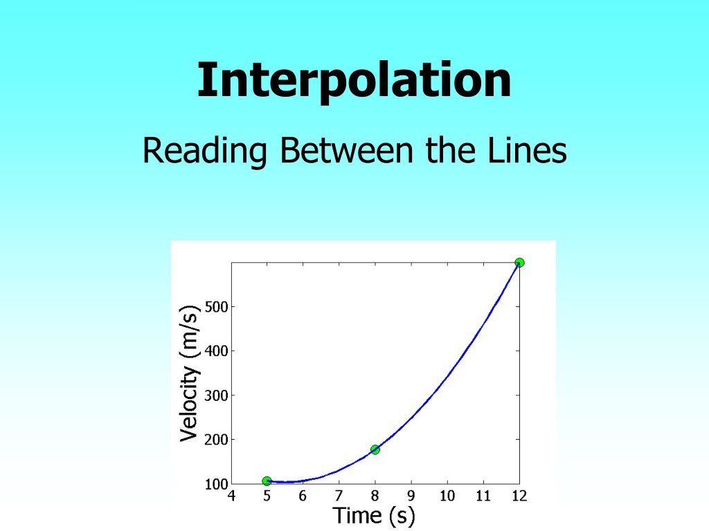
Interpolation Reading Between the Lines
WHAT IS INTERPOLATION ? Given (x0,y0), (x1,y1), (xn,yn), find the value of y at a value of x that is not given. Figure Interpolation of discrete data. http://nm.mathforcollege.com
FLY ROCKET FLY, FLY ROCKET FLY The upward velocity of a rocket is given as a function of time in table below. Find the velocity and acceleration at t=16 seconds. Table Velocity as a function of time. ? ? , m/s ?, s 0 0 10 227.04 15 362.78 20 517.35 22.5 602.97 30 901.67 Velocity vs. time data for the rocket example
SPECIFIC HEATOF CARBON A carbon block is heated up from room temperature of 300K to 1800K. How much heat is required to do so? Specific Heat (J/kg-K) Temperature (K) 200 420 400 1070 600 1370 1000 1820 1500 2000 2000 2120
THERMISTOR CALIBRATION Thermistors are based on change in resistance of a material with temperature. A manufacturer of thermistors makes the following observations on a thermistor. Determine the calibration curve for thermistor. R ( ) T( C) 1101.0 911.3 636.0 451.1 25.113 30.131 40.120 50.128
FOLLOWTHE CAM A curve needs to be fit through the given points to fabricate the cam. 4 3 5 2 6 Point 1 2 3 4 5 6 7 x (in.) 2.20 1.28 0.66 0.00 0.60 1.04 1.20 y (in.) 0.00 0.88 1.14 1.20 1.04 0.60 0.00 Y 1 X 7 Cam Profile 1.4 1.2 1 0.8 y 0.6 0.4 0.2 0 -2 -1 0 1 2 3 x
Spline Interpolation Method Major: All Engineering Majors Authors: Autar Kaw, Jai Paul http://numericalmethods.eng.usf.edu Transforming Numerical Methods Education for STEM Undergraduates http://numericalmethods.eng.usf.edu 8
Spline Method of Interpolation http://nm.MathForCollege.com
Why Splines ? 1 ?(?) = 1 + 25?2 Table : Six equidistantly spaced points in [-1, 1] 1 = y x + 2 1 25 x -1.0 0.038461 -0.6 0.1 -0.2 0.5 0.2 0.5 0.6 0.1 Figure : 5th order polynomial vs. exact function 1.0 0.038461 http://numericalmethods.eng.usf.edu 10
Why Splines ? 1.2 0.8 0.4 y 0 -1 -0.5 0 0.5 1 -0.4 -0.8 x 19th Order Polynomial f (x) 5th Order Polynomial Figure : Higher order polynomial interpolation is a bad idea 11
Linear Spline Interpolation Given ( ) ( , ) ( )( ) , , ,......, , , , fit linear splines to the data. This simply involves x y x y x y x y 0 0 1 1 1 1 n n n n forming the consecutive data through straight lines. So if the above data is given in an ascending order, the linear splines are given by ( ) ) ( i i x f y = Figure : Linear splines 12
Linear Spline Interpolation (contd) ( ) ( ) f x f x = + 1 x 0 ( ) ( ) ( ), f x f x x x x x x 0 0 0 1 x 1 0 ( ) ( ) f x f x = + 2 x 1 ( ) ( ), f x x x x x x 1 1 1 2 x 2 1 . . . ( ) ( ) f x f x = + 1 n n ( ) ( ), f x x x x x x 1 1 1 n n n n x x 1 n n Note the terms of ( ) ( 1) f x f x i i x x 1 i i in the above function are simply slopes between ix and ix . 1 13
Example The upward velocity of a rocket is given as a function of time in Table 1. Find the velocity at t=16 seconds using linear splines. Table Velocity as a function of time (s) (m/s) 0 227.04 362.78 517.35 602.97 901.67 ?(?) ? 0 10 15 20 22.5 30 Figure. Velocity vs. time data for the rocket example 14
Linear Spline Interpolation 0= (0 = t 15 , ) 362 78 . t v 550 517.35 1= t (1= t 20 , ) 517 35 . v 500 ( ) ( ) v t v t = + 1 t 0 ( ) ( ) ( ) v t v t t t 0 0 t ys 1 0 f range ( ( ) 450 517 35 . 362 78 . ) f xdesired = + 362 78 . ( 15 ) t t 20 15 15 400 = + ( ) 362 78 . 30 913 . ( ) v t = At 16 , t 362.78 350 10 xs0 12 14 16 18 xdesired 20 22 24 xs1 = + 16 ( ) 362 = 78 . 30 913 . 16 ( 15 ) v xsrange + 10 10 393 7 . m/s 15
Quadratic Spline Interpolation Given ( ) ( , ) ( ) ( , ) , , ,......, , , , fit quadratic splines through the data. The splines x y x y x y x y 0 0 1 1 1 1 n n n n are given by = + + 2 ( ) , f x a x b x c x x x 1 1 1 0 1 = + + 2 , a x b x c x x x 2 2 2 1 2 . . . = + + 2 , a x b x c x x x 1 n n n n n = Find , , , 1, 2, , n ia ib ic i 16
Quadratic Spline Interpolation (contd) Each quadratic spline goes through two consecutive data points 2 + + = ( ) a x b x c f x 1 0 1 0 1 0 2 + + = ( ) . a x b x c f x 1 1 1 1 1 1 . . 2 + + = ( ) a x b x c f x 1 1 1 i i i i i i 2 + + = ( ) . a x b x c f x i i i i i i . . 2 + + = ( ) a x b x c f x 1 1 1 n n n n n n 2 + + = ( ) a x b x c f x n n n n n n This condition gives 2n equations 17
Quadratic Spline Interpolation (contd) The first derivatives of two quadratic splines are continuous at the interior points. For example, the derivative of the first spline + + + 2 is 2 a x b x c a x b 1 1 1 1 1 The derivative of the second spline + + + 2 is 2 a x b x c a x b 2 2 2 2 2 x = and the two are equal at giving 1x + = + 2 2 a x b a x b 1 1 1 2 1 2 + = 2 2 0 a x b a x b 1 1 1 2 1 2 18
Quadratic Spline Interpolation (contd) Similarly at the other interior points, + = 2 2 0 a x b a x b 2 2 2 3 2 3 . . . + = 2 2 0 a x b a x b + + 1 1 i i i i i i . . . + = 2 2 0 a x b a x b 1 1 1 1 n n n n n n + ) 1 = ) 1 We have (n-1) such equations. The total number of equations is 2 ( ) ( 3 ( . n n n 1= a We can assume that the first spline is linear, that is 0 19
Quadratic Spline Interpolation (contd) This gives us 3n equations and 3n unknowns. Once we find the 3n constants, we can find the function at any value of x using the splines, = + + 2 ( ) , f x a x b x c x x x 1 1 1 0 1 = + + 2 , a x b x c x x x 2 2 2 1 2 . . . = + + 2 , a x b x c x x x 1 n n n n n 20
Quadratic Spline Example The upward velocity of a rocket is given as a function of time. Using quadratic splines a) Find the velocity at t=16 seconds b) Find the acceleration at t=16 seconds c) Find the distance covered between t=11 and t=16 seconds t s 0 10 15 20 22.5 30 v(t) m/s 0 227.04 362.78 517.35 602.97 901.67
Data and Plot t s 0 10 15 20 22.5 30 v(t) m/s 0 227.04 362.78 517.35 602.97 901.67
Solution ?(?) = ?1?2+ ?1? + ?1, 0 ? 10 = ?2?2+ ?2? + ?2, 10 ? 15 = ?3?2+ ?3? + ?3, 15 ? 20 = ?4?2+ ?4? + ?4, 20 ? 22.5 = ?5?2+ ?5? + ?5, 22.5 ? 30 Let us set up the equations
Each Spline Goes Through Two Consecutive Data Points ?(?) = ?1?2+ ?1? + ?1, 0 ? 10 ?1(0)2+ ?1(0) + ?1= 0 ?1(10)2+ ?1(10) + ?1= 227.04
Each Spline Goes Through Two Consecutive Data Points t s 0 v(t) m/s 0 227.04 362.78 517.35 602.97 901.67 ?2(10)2+ ?2(10) + ?2= 227.04 ?2(15)2+ ?2(15) + ?2= 362.78 ?3(15)2+ ?3(15) + ?3= 362.78 10 15 20 22.5 30 ?3(20)2+ ?3(20) + ?3= 517.35 ?4(20)2+ ?4(20) + ?4= 517.35 ?4(22.5)2+ ?4(22.5) + ?4= 602.97 ?5(22.5)2+ ?5(22.5) + ?5= 602.97 ?5(30)2+ ?5(30) + ?5= 901.67
Derivatives are Continuous at Interior Data Points ?(?) = ?1?2+ ?1? + ?1, 0 ? 10 = ?2?2+ ?2? + ?2, 10 ? 15 ? ???1?2+ ?1? + ?1 ? ???2?2+ ?2? + ?2 = ?=10 ?=10 2?1? + ?1 ?=10= 2?2? + ?2 ?=10 2?110 + ?1= 2?210 + ?2 20?1+ ?1 20?2 ?2= 0
Derivatives are continuous at Interior Data Points At t=10 2?1(10) + ?1 2?2(10) ?2= 0 At t=15 2?2(15) + ?2 2?3(15) ?3= 0 At t=20 2?3(20) + ?3 2?4(20) ?4= 0 At t=22.5 2?4(22.5) + ?4 2?5(22.5) ?5= 0
Last Equation ?1= 0
Final Set of Equations ?1 ?1 ?1 ?2 ?2 ?2 ?3 ?3 ?3 ?4 ?4 ?4 ?5 ?5 ?5 0 0 1 1 0 0 0 0 0 0 0 0 0 0 0 0 0 0 0 0 0 10 15 0 0 0 0 0 0 1 1 0 0 0 0 0 1 1 0 0 0 0 0 0 0 0 0 0 0 0 0 0 0 0 0 0 0 0 0 0 0 1 1 0 0 0 0 0 0 0 0 0 0 0 0 0 0 0 0 0 0 0 0 0 20 22.5 0 0 0 0 1 1 0 0 0 0 0 0 0 1 1 0 0 0 0 0 0 0 0 0 0 0 0 0 0 0 0 0 0 0 0 0 0 0 0 0 0 0 0 0 0 0 1 1 0 0 0 0 0 0 100 0 0 0 0 0 0 0 0 20 0 0 0 1 10 0 0 0 0 0 0 0 0 1 0 0 0 0 227.04 227.04 362.78 362.78 517.35 517.35 602.97 602.97 901.67 0 0 0 0 0 100 225 0 0 0 0 0 0 20 30 0 0 0 225 400 0 0 0 0 0 30 40 0 0 15 20 0 0 0 0 0 1 1 0 0 400 506.25 0 0 0 0 40 45 0 = 506.25 900 0 0 0 45 0 22.5 30 0 0 0 1 0
?? ?? ?? Coefficients of Spline i 1 2 3 4 5 ai 0 bi ci 0 22.704 4.928 35.66 -33.956 28.86 0.8888 -0.1356 1.6048 0.20889 88.88 -141.61 554.55 -152.13
Final Solution ?(?) = 22.704?, 0 ? 10 = 0.8888?2+ 4.928? + 88.88, 10 ? 15 = 0.1356?2+ 35.66? 141.61, 15 ? 20 = 1.6048?2 33.956? + 554.55, 20 ? 22.5 = 0.20889?2+ 28.86? 152.13, 22.5 ? 30
Velocity at a Particular Point a) Velocity at t=16 ?(?) = 22.704?, 0 ? 10 = 0.8888?2+ 4.928? + 88.88, 10 ? 15 = 0.1356?2+ 35.66? 141.61, 15 ? 20 20 ? 22.5 = 1.6048?2 33.956? + 554.55, 22.5 ? 30 = 0.20889?2+ 28.86? 152.13, ? 16 = 0.1356 162+ 35.66 16 141.61 = 394.24m/s
Acceleration from Velocity Profile b) Acceleration at t=16 0 ? 10 ?(?) = 22.704?, = 0.8888?2+ 4.928? + 88.88, 10 ? 15 = 0.1356?2+ 35.66? 141.61, 15 ? 20 = 1.6048?2 33.956? + 554.55, 20 ? 22.5 = 0.20889?2+ 28.86? 152.13, 22.5 ? 30 ?(16) =? ?(?) ?? ?=16
Acceleration from Velocity Profile The quadratic spline valid at t=16 is given by ? ? = 0.1356?2+ 35.66? 141.61,15 ? 20 , ?(?) =? ??( 0.1356?2+ 35.66? 141.61) = 0.2712? + 35.66, 15 ? 20 ?(16) = 0.2712(16) + 35.66 = 31.321m/s2
Distance from Velocity Profile c) Find the distance covered by the rocket from t=11s to t=16s. 0 ? 10 ?(?) = 22.704?, = 0.8888?2+ 4.928? + 88.88, 10 ? 15 = 0.1356?2+ 35.66? 141.61, 15 ? 20 = 1.6048?2 33.956? + 554.55, 20 ? 22.5 = 0.20889?2+ 28.86? 152.13, 22.5 ? 30 16 ? 16 ? 11 = ?(?)?? 11
Distance from Velocity Profile ? ? = 0.8888?2+ 4.928? + 88.88, 10 ? 15 = 0.1356?2+ 35.66? 141.61, 15 ? 20 16 15 16 ? 16 ? 11 = ?(?)?? = ?(?)?? + ?(?)?? 11 11 15 15 (0.8888?2+ 4.928? + 88.88)?? = 11 16 ( 0.1356?2+ 35.66? 141.61)?? + 15 = 1595.9m
END http://numericalmethods.eng.usf.edu
Find a Smooth Shortest Path for a Robot http://numericalmethods.eng.usf.edu
Points for Robot Path x y 2.00 4.5 5.25 7.81 9.20 10.60 7.2 7.1 6.0 5.0 3.5 5.0 ? ? Find the shortest but smooth path through consecutive data points
Compare Spline & Polynomial Interpolant Path Length of path Polynomial Interpolant=14.9 Spline Interpolant =12.9
