Understanding Inferential Statistics and Hypothesis Testing in Research
Inferential statistics in research involve estimating population parameters from sample statistics and making decisions based on probability. Researchers follow a set process, starting with preparing for a study, defining variables, stating hypotheses, selecting appropriate tests, analyzing data, and making conclusions. The key to forming testable hypotheses is specifying a relationship between variables that can be empirically tested. Examples include directional and non-directional hypotheses to predict outcomes in a study.
Download Presentation

Please find below an Image/Link to download the presentation.
The content on the website is provided AS IS for your information and personal use only. It may not be sold, licensed, or shared on other websites without obtaining consent from the author. Download presentation by click this link. If you encounter any issues during the download, it is possible that the publisher has removed the file from their server.
E N D
Presentation Transcript
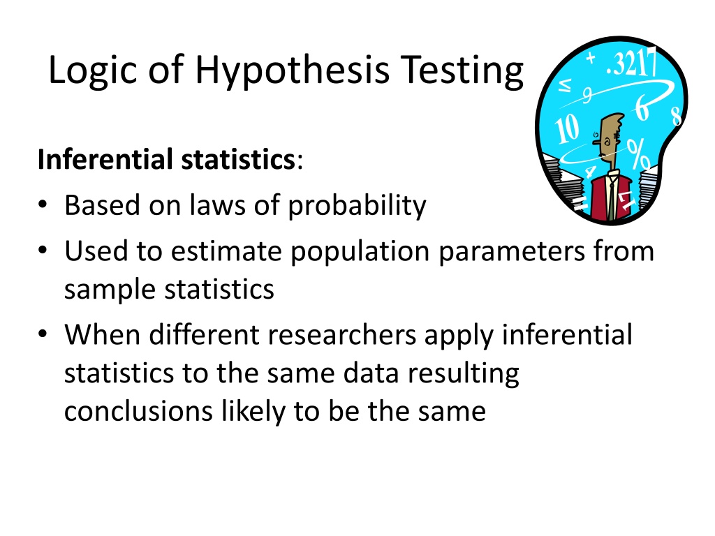
Logic of Hypothesis Testing Inferential statistics: Based on laws of probability Used to estimate population parameters from sample statistics When different researchers apply inferential statistics to the same data resulting conclusions likely to be the same
Basic Preparation Planning a Research Study Identify problem Review literature Determine conceptual and operational definitions of variables Select appropriate instruments
Basic Steps Making Inferential Decisions Five basic steps in making inferential decisions: 1. State hypotheses 2. Select appropriate inferential statistic(s) 3. Specify alpha or level of significance 4. Data analysis 5. Decision-making
Basic Steps: Step 1 Step 1 Hypotheses: Prior to data collection: Delineate study purpose Prepare formal purpose statement in form of a hypothesis Essential conditions for a testable hypothesis: Must delineate a relationship between variables Relationship must be empirically testable through the collection of data
Step 1 Essential Conditions for Testable Hypothesis: Must make a clear statement regarding explicit nature or posited relationship between the variables Decide before study conducted whether or not to use a directional hypothesis (one-tailed) or non directional (two-tailed) Examples testable hypotheses Null (HO): There is no difference between staff nurses participating in a mentoring program and those not participating with respect to job satisfaction
Step 1 Examples Testable Hypotheses: Directional research hypothesis (HA, alternate hypothesis): Staff nurses participating in a mentoring program will have significantly higher job satisfaction than staff nurses not participating in a mentoring program Non directional research hypothesis: There will be a significant difference between job satisfaction of staff nurses participating in a mentoring program and staff nurses not participating in a mentoring program.
Step 1 Testable Hypotheses There is no significant relationship between age and blood pressure There is no significant difference between students receiving and those not receiving instruction with respect to achievement scores An individual s blood pressure is a function of his age, weight and daily exercise regime Un testable Hypotheses There is no significant difference between age and blood pressure Administering instruction is the best way to increase student achievement scores What is the relationship between an individual s blood pressure and his age, weight and daily exercise regime ?
Step 1 Is the following hypothesis testable? Why or why not? A researcher hypothesizes that Group A is significantly better than groups B and C and group B is better than group C. Adapted from: Waltz,C.F. & Bausell, R.B. (1981) Nursing Research: Design, Statistics and Computer Analysis. 17-19. Philadelphia: F.A. Davis Company
Basic Steps: Step 2 Step 2 Selecting the appropriate inferential statistic(s) prior to data collection Types of statistical tests: parametric & non parametric Parametric tests have the following characteristics: Involve estimation of a parameter Require interval or ratio levels of measurement Involve a set of assumptions to be met (e.g. that the variables are normally distributed in the population) Parametric tests are more powerful than nonparametric tests , thus are usually preferred
Step 2 Nonparametric tests Do not estimate parameters Involve less restrictive assumptions about the distribution shape (referred to as distribution free tests) Use when Variables are not at the interval or ratio level distribution is markedly skewed (i.e. not normal) when sample size is small
Step 2 Research data is used to compute test statistics Every test statistic is based on a related theoretical distribution Value of the computed statistic is compared to values that specify critical limits for the underlying distribution When beyond the critical limit the results are said to be statistically significant (vs clinically significant) Stat significance means that the obtained results are not likely to have been a result of chance at some specified level, e.g., <.05 . A nonsignificant result could reflect chance fluctuations.
Factors considered in selecting a test statistic include: Levels of measurement of the variables Whether a parametric test is justified Whether dependent or independent groups Whether the focus is correlations or group comparisons and if so, How many groups are being compared
Step 2 Types of comparisons: Between subjects design Comparisons involve different subjects (e.g. experimental and control group) and Statistical test is for independent groups Within subjects design Involve one group of subjects who are exposed to two or more treatments (e.g. staff nurse job satisfaction measured, same staff nurses participate in a mentoring program and job satisfaction measured again ) Comparisons are not independent because the same subjects used in both conditions, thus referred to as tests for dependent groups
Basic Steps: Step 3 Step 3 Specifying alpha or level of significance Typically researcher sets alpha at 0.05. However there are instances when researcher may decide to use a more stringent level of alpha , e.g. 0.01. Alpha 0.05 indicates researcher willing to take up to 5% risk of making an error (Type I error) when deciding statistical significance. Alpha 0.01 indicates researcher willing to take up to 1% risk of Type I error Type I error occurs when a researcher rejects the null hypothesis when in fact it is true in the population.
Alpha, Beta, Power, Effect Size Null is true Null is false 1 Beta Power Researcher calc and decides the null is false: Reject null Alpha Type I error False positive CORRECT REJECTION Researcher calc and decides the null is true: Null accepted Beta 1 Alpha Type II error False negative CORRECT NON-REJECTION Alpha Level of significance, p value often set at 0.05 or 0.01 Type I error-Reject a null hypothesis when it is true Beta Type II error-Fail to reject null hypothesis when it is false One controls the risk of a type I error by selecting a level of significance. Reducing the alpha to .01 from .05 reduces type I error Lowering the risk of Type I increases the risk of Type II. Simplest way to reduce type II errors is to increase sample size.
Basic Steps: Step 4 Step 4 Data analysis Data entered into computer in a DATA file SPSS used to analyze the results SPSS Printout includes all necessary descriptive / inferential statistics including level of significance or probability.
Step 4 Example : Data Analysis Suppose: A researcher is interested in the correlation between subjects years of experience as a staff nurse and scores on a job satisfaction questionnaire (sample size, n=700) . The researcher employs the Pearson correlation coefficient (rxy) for this analysis and the following SPSS results are obtained.
Correlations Years exp. Job sat. Years exp. Correlation 1.00 .384** Sig. (1-tailed) .000 N 700 699 _______________________________________ Job sat. Correlation .384** 1.00 Sig. (1-tailed) .000 N 699 700 ** Correlation significant at 0.01 level (1-tailed)
Step 4 Example: Data Analysis The p value (or level of significance) gives the probability of committing error if results are declared to be statistically significant. In this example, Sig.(1-tailed) for the correlation between years of experience and job satisfaction <.001 (=.000), indicating the result is statistically significant. Whether a test is 1-tailed or 2-tailed is determined on the basis of the hypothesis statement
Basic Steps: Step 5 Step 5. Making a decision involves: Do you reject or fail to reject the null hypothesis? The decision is made by examining the p level furnished by the computer. Example: if the alpha level is set at .05, inferential statistics with p levels of .05 or less are statistically significant. When this is the case , the HO is rejected and HA is supported.
Step 5 The researcher might report the results of the data analysis example as follows: There was a significant correlation (r=.38, p =.01, 1-tailed) between years of experience and job satisfaction for the 699 subjects. In reporting correlation results the coefficient is rounded to 2 decimal places
Step 5 The inferential statistic employed is based on the data collected in the study. This inferential statistic is referred to as the test statistic ( i.e. it tests the null hypothesis) The test statistic is also called the obtained or calculated statistic. Each inferential statistic ( e.g. t-test, chi-square) has a separate table of what are referred to as critical values (CVs). The values of the computed test statistic are compared to expected values (critical values) provided in tables or calculated in the memory of the computer
Step 5 The appropriate table of CVs can be found in most statistics text books.[appendix pgs 747-752] When employing the CV in the appropriate table for decision making, the general rule is: If the test statistic calculated for the data in your study equals or exceeds the CV, then the result is determined to be statistically significant (p< .05 or .01) CVs are usually not included in research reports, instead the p level is included in reports.
Step 5 Examples of decision making using CVs Test statistic = 4.11; CV= 4.110; decision: result is statistically significant because it equals the CV Test statistic = 4.11; CV = 4.120; decision: result not statistically significant because it is less than the CV Test statistic = 4.11; CV = 3.98; decision: result is statistically significant because it exceeds the CV
Step 5 Ex: Interpreting and Reporting Hypothesis Testing Results Given an alpha level of .01 Suppose the results are statistically significant, that is, p<.01. This means that getting this result by chance is less than 1 time in 100. Therefore , the null hypothesis is rejected. The evidence supports the research hypothesis That is, if your were testing for a difference in group means , statistical significance would lead you to conclude that the difference is not due to chance.
Step 5 Suppose the results are non significant ( i.e. p> .01). This means that: The null hypothesis cannot be rejected The evidence fails to support the research hypothesis That is, if you were testing a difference in group means , statistical non significance would lead you to conclude that the apparent difference in group means is presumably due to chance. Non significantly different means are treated as if they were equal.
Type I error (also known as alpha error): researcher REJECTs the null hypothesis (HO) when it is true in the population. Type II error (also known as beta error): researcher FAILS to reject the null hypothesis (HO) when it is FALSE in the population The actual situation is that the null hypothesis is: _____________________________________ TrueFalse True Correct Type II Error (Null accepted) Decision Beta _______________________________________ False Type I Error Correct Decision (Null rejected) Alpha
Step 5 Power refers to the probability that the statistical procedure will be able to reject a false null hypothesis. That is, the probability that the researcher will not make a Type II error. Power depends on Alpha : for example, alpha set at .05 gives more power as compared to an alpha set at .01 or .001
power Sample size: the larger the sample the more power Effect size: strength of the study s expected effect (in experimental research); expected difference (in descriptive comparative research); expected correlation (in descriptive correlational research ). Parametric statistics are generally more powerful than nonparametric For some statistics (e.g. t-test) , one-tailed hypotheses (tests) are more powerful than two-tailed tests , PROVIDED the researcher predicts the right direction Power for a study should be at .80 or higher
