Understanding Hypothesis Evaluation in Machine Learning
Evaluating hypotheses in machine learning is crucial for assessing accuracy and making informed decisions. This process involves estimating hypothesis accuracy, sampling theory basics, deriving confidence intervals, comparing learning algorithms, and more. Motivated by questions about accuracy estimation, hypothesis comparison, and efficient data utilization, this chapter explores methods for evaluating hypotheses and understanding bias and variance in model skill estimation.
Download Presentation

Please find below an Image/Link to download the presentation.
The content on the website is provided AS IS for your information and personal use only. It may not be sold, licensed, or shared on other websites without obtaining consent from the author. Download presentation by click this link. If you encounter any issues during the download, it is possible that the publisher has removed the file from their server.
E N D
Presentation Transcript
Evaluating Hypotheses is divided into 7parts they are as follows: 5.1. Motivation 5.2. Estimating Hypothesis Accuracy 5.3. Basics of Sampling Theory 5.4. A General Approach for Deriving Confidence Intervals 5.5. Difference in Error of Two Hypotheses 5.6. Comparing Learning Algorithms 5.7. Summary and Further Reading
Motivation The chapter starts off by stating the importance of evaluating hypotheses in machine learning Empirically evaluating the accuracy of hypotheses is fundamental to machine learning. The chapter is motivated by three questions; they are: Given the observed accuracy of a hypothesis over a limited sample of data, how well does this estimate its accuracy over additional examples? Given that one hypothesis outperforms another over some sample of data, how probable is it that this hypothesis is more accurate in general? When data is limited, what is the best way to use this data to both learn a hypothesis and estimate its accuracy? All three questions are closely related. The first question raises concerns over errors in the estimate of model skill and motivates the need for confidence intervals. The second question raises concerns about making decisions based on model skill on small samples and motivates statistical hypothesis testing. And finally, the third question considers the economical use of small samples and motivates resampling methods such as k-fold cross-validation.
This chapter discusses methods for evaluating learned hypotheses, methods for comparing the accuracy of two hypotheses, and methods for comparing the accuracy of two learning algorithms when only limited data is available. The motivation closes with a reminder of the difficulty of estimating the skill of a hypothesis. Specifically the introduction of bias and variance in the estimate of the skill of a model: Bias in the estimate. When the model is evaluated on training data, overcome by evaluating the model on a hold out test set. Variance in the estimate. When the model is evaluated on an independent test set, overcome by using larger tests sets.
Estimating Hypothesis Accuracy The skill or prediction error of a model must be estimated, and as an estimate, it will contain error. This is made clear by distinguishing between the true error of a model and the estimated or sample error. One is the error rate of the hypothesis over the sample of data that is available. The other is the error rate of the hypothesis over the entire unknown distribution D of examples.
Sample Error. Estimate of true error calculated on a data sample. True Error. Probability that a model will misclassify a randomly selected example from the domain. We want to know the true error, but we must work with the estimate, approximated from a data sample. This raises the question of how good is a given estimate of error? One approach is to calculate a confidence interval around the sample error that is large enough to cover the true error with a very high likelihood, such as 95%. Assuming that the error measure is a discrete proportion, such as classification error, the calculation of the confidence interval is calculated as follows: Calculation of Confidence Interval for Classification Error. Where error_s is the sample error, n is the total number of instances in the test set used to calculate the sample error and 1.96 is the critical value from the Gaussian distribution for a likelihood of 95%.
Error Estimation and Estimating Binomial Proportions The Binomial Distribution Definition: Consider a random variable Y that takes on the possible values yl, . . . yn. The expected value of Y, E[Y], is
Definition: The variance of a random variable Y, Var[Y], is Var[Y] = E[(Y - E[Y])2] Definition: The standard deviation of a random variable Y, ?y, is
Estimators, Bias, and Variance In general, given r errors in a sample of n independently drawn test examples, the standard deviation for errors(h) is given by
which can be approximated by substituting rln = errors(h) for p
for N% confidence intervals for discrete- valued hypotheses
A General Approach for Deriving Confidence Intervals Given the equation to calculate the confidence intervals for proportional values and the statistical reasoning behind the equation, a general procedure is presented to calculate confidence intervals. The procedure is summarized below.
Central Limit Theorem The Central Limit Theorem is a very useful fact because it implies that whenever we define an estimator that is the mean of some sample (e.g., errors(h) is the mean error), the distribution governing this estimator can be approximated by a Normal distribution for sufficiently large n. Consider a set of independent identically distributed random variables Y1 .Yn governed by an arbitrary probability distributionwith mean and finite variance 2 .define the sample mean
Difference in Error of Two Hypotheses This section looks at applying the general procedure for calculating confidence intervals to the estimated difference in classification error between two models. The approach assumes that each model was trained on a different independent sample of the data. Therefore, the calculation of the confidence interval in the difference in error between the two models adds the variance from each model. In some cases we are interested in the probability that some specific conjecture is true, rather than in confidence intervals for some parameter.
Comparing Learning Algorithms When we train a model, there are tons of learning algorithms that can be used to train the model correctly, and we ll want to choose the algorithm that best fits the universal dataset(training and testing dataset). To find the best learning algorithm, we compare different learning algorithms. In this blog, we ll have a look at some parameters we need to keep in my to compare learning algorithms. Why rely on Statistical methods to compare learning algorithms? The mean performance of machine learning models is commonly calculated using k-fold cross-validation. The algorithm with the best average performance should outperform those with the worst average performance. But what if the discrepancy in average performance is due to a statistical anomaly? To determine whether the difference in mean performance between any two algorithms is real or not, a statistical hypothesis test is used.
Comparing of learning Algorithms: We want to know which of the Learning algorithm is the better learning approach for learning a specific target function f on average. Average the performance of these two algorithms over all the training sets of size n selected from the instance distribution D. We use this formula to estimate the expected value of the difference in the errors. Where L(S) signifies the hypothesis generated by learning technique L given a sample of training data of size S. When comparing learning algorithms, we only have a small sample Do of data to work with.
Do can be divided into two sets: a training set So and a disjoint test set To. The test data can be used to assess the accuracy of the two hypotheses, while the training data can be used to train both LA and LB (the learning algorithms).
There are two major distinctions between this estimator and the quantity in Equation (5.14): To begin, we ll use error(h) to approximate errorD(h). Second, rather than considering the anticipated value of this difference overall samples S chosen from the distribution D, we just measure the difference in errors for one training set S0. To make the estimator in Equation better (5.15) split the data on a regular basis and take the mean of the test set errors for these individual studies and divide them into disjoint training and test sets.
The quantity returned by the procedure of Table 5.5 can be taken as an estimate of the desired quantity from Equation 5.14. More appropriately, we can view as an estimate of the quantity. Where S represents a random sample of size ((k-1)/k)*|D0| drawn uniformly from D0. The approximate N% confidence interval for estimating the quantity in Equation 5.16 using is given by Where tN, k-1 is a constant that plays a role analogous to that of Zn in our earlier confidence interval expressions, and where is an estimate of the standard deviation of the distribution governing . In particular, defined as is
Notice the constant tN,k-1 in equation (5.17) has two subscripts. The first one specifies the desired confidence level, as it did for our earlier constant zN. The second parameter called the number of degrees of freedom and usually denoted by v, is related to the number of independent random events that go into producing the value for the random variable . The number of degrees of freedom is k-1. Table 5.6 contains the selected values for the parameter t. Notice that as k -> , the value of tN, k- 1 approaches the constant zN.
Paired tests are tests in which the hypotheses are assessed over identical samples. Because any variations in observed errors are related to differences between the hypotheses, paired tests often provide tighter confidence ranges. Paired t-Tests: Consider the following estimation problem to better understand the justification for the confidence interval estimate given by Equation (5.17): The observed values of a collection of independent, identically distributed random variables Y1, Y2, , Yk are presented to us. We want to figure out what the mean of the probability distribution that governs this Yi is. The sample mean will be our estimator.
the individual Yi follow a Normal distribution. In this idealized method, we modify the procedure of Table 5.5. Instead of drawing from the fixed sample Do. Each iteration through the loop generates a new random training set Si and a new random test set Ti by pulling from the underlying instance distribution. In particular, the ?? measured by the procedure now correspond to the independent, identically distributed random variables Yi. The mean ? of their distribution corresponds to the expected difference in error between the two learning methods [i.e., Equation (5.14)]. The sample means ? is the quantity (? ) computed by this idealized version of the method.
The t distribution is a bell-shaped distribution similar to the Normal distribution, but wider and shorter to reflect the greater variance introduced by using s. To approximate the true standard deviation ?. The t distribution approaches the Normal distribution when k approaches infinity.
Practical considerations In contrast the K-fold method is limited by the total number of examples, by the use of each example only once in a test set , and by our desire to use samples of size at least 30. In contrast , the test sets generated by K-fold cross validation are independent because each instance is included in only one test set.


