Understanding Complexity Measures of Boolean Functions
This work delves into the intricate world of complexity measures for Boolean functions, exploring concepts such as certificate complexity, decision tree depth, sensitivity, block sensitivity, PRAM complexity, and more. It sheds light on the relationships among different complexity measures and provides insights into fundamental results in Boolean function complexity theory. The study also revisits complexity classes, computational perspectives, and the sensitivity conjecture, offering a high-level summary of the computational viewpoint on this classic open question. Through examples and theorems, the connection between decision tree depth and real degree in polynomial time is showcased.
- Boolean Functions
- Complexity Measures
- Decision Trees
- Sensitivity Conjecture
- Computational Perspective
Download Presentation

Please find below an Image/Link to download the presentation.
The content on the website is provided AS IS for your information and personal use only. It may not be sold, licensed, or shared on other websites without obtaining consent from the author. Download presentation by click this link. If you encounter any issues during the download, it is possible that the publisher has removed the file from their server.
E N D
Presentation Transcript
Smooth Boolean Functions are Easy: Efficient Algorithms for Low-Sensitivity Functions Rocco Servedio Joint work with Parikshit Gopalan (MSR) Noam Nisan (MSR / Hebrew University) Kunal Talwar (Google) Avi Wigderson (IAS) ITCS 2016
The star of our show: f: {0,1}n {0,1}
Complexity and Boolean functions Complexity measures: combinatorial/analytic ways to get a handle on how complicated f is Certificate complexity Decision tree depth (deterministic, randomized, quantum) Sensitivity Block sensitivity PRAM complexity Real Polynomial degree (exact, approximate) All lie in {0,1, ,n} for n-variable Boolean functions.
Complexity and Boolean functions revisited Complexity classes: computationalways to get a handle on how complicated f is Unrestricted circuit size Unrestricted formula size AC0 circuit size DNF size All lie in {0,1, ,2n} for n-variable Boolean functions.
High-level summary of this work: A computational perspective on a classic open question about complexity measures of Boolean functions . ...namely, the sensitivity conjecture of [NisanSzegedy92].
Background: Complexity measures Certificate complexity Decision tree depth (deterministic, randomized, quantum) Block sensitivity PRAM complexity Real Polynomial degree (exact, approximate) Fundamental result(s) in Boolean function complexity: For any Boolean function f, the above complexity measures are all polynomially related to each other.
Examples: DT-depth and real degree DT-depth(f) = minimum depth of any decision tree computing f DT-depth is 4 1 0 1 0 1 1 0 1 degR(f) = degree of the unique real multilinear polynomial computing f: {0,1}n {0,1}
DT-depth and real degree are polynomially related Theorem: [NisanSzegedy92,NisanSmolensky,Midrijanis04] For any Boolean function f, _ _ degR(f) < DT-depth(f) < 2degR(f)3. (Lower bound is trivial: for each 1-leaf at depth d, have degree-d polynomial outputing 1 iff its input reaches that leaf, else 0. Sum these.) Polynomial for this leaf: x1x2(1-x4)x3 1 0 1 0 1 1 0 1
An outlier among complexity measures: Sensitivity s(f,x) = sensitivity of f at x = number of neighbors y of x such that f(x) = f(y) s(f) = (max) sensitivity of f = max of s(f,x) over all x in {0,1}n / _ Folklore: s(f)< DT-depth(f). 1 0 1 0 1 1 0 1 Question: [Nisan91,NisanSzegedy92] _ Is DT-depth(f) < poly(s(f))?
The sensitivity conjecture _ Conjecture: DT-depth(f) < poly(s(f)). Equivalently, block sensitivity, certificate complexity, real degree, approximate degree, randomized/quantum DT-depth Despite much effort, best known upper bounds are exponential in sensitivity: [Simon82]: # relevant variables < s(f)4s(f) [KenyonKutin04]: bs(f) < es(f) [AmbainisBavarianGaoMaoSunZuo14]: bs(f),C(f) < s(f)2s(f)-1, deg(f) < 2s(f)(1+o(1)) [AmbainisPrusisVihrovs15]: bs(f) < (s(f)-1/3)2s(f)-1 _ _ _ _ _
This work: Computational view on the sensitivity conjecture _ Conjecture: DT-depth(f) < poly(s(f)). Previous approaches: combinatorial/analytic But conjecture also is a strong computational statement: low-sensitivity functions are very easy to compute!
_ Conjecture: DT-depth(f) < poly(s(f)). Conjecture implies Prior to this work, even seems not to have been known. In fact, even an upper bound on the # of sensitivity-s functions seems not to have been known.
Results Theorem: Every n-variable sensitivity-s function is computed by a Boolean circuit of size nO(s). In fact, every such function is computed by a Boolean formula of depth O(s log(n)). So now the picture is ? ? ? ?
Results (continued) Circuit/formula size bounds are consequences of the conjecture. Another consequence of the conjecture: Theorem: Any n-variable sensitivity-s function can be self- corrected from 2-cs-fraction of worst-case errors using nO(s) queries and runtime. (Conjecture low-sensitivity f has low degR has low deg2 has self-corrector) All results are fairly easy. (Lots of directions for future work!)
Simple but crucial insight Fact: If f has sensitivity s, then f(x) is completely determined once you know f s value on 2s+1 neighbors of x. f(x)=? x 2s+1 neighbors f(x)=1 .. neighbors where f=0 neighbors where f=1 Either have at least s+1 many 0-neighbors or at least s+1 many 1-neighbors. The value of f(x) must equal this majority value! (If it disagreed, would have s(f) > s(f,x) > s+1.) _ _
Theorem: Every sensitivity-s function on n variables is uniquely specified by its values on any Hamming ball of radius 2s. 1n weight level 2s+1; each point here has 2s+1 down-neighbors ? weight levels 0, ,2s 0n
Theorem: Every sensitivity-s function on n variables is uniquely specified by its values on any Hamming ball of radius 2s. 1n weight level 2s+1; each point here has 2s+1 down-neighbors weight levels 0, ,2s 0n
Theorem: Every sensitivity-s function on n variables is uniquely specified by its values on any Hamming ball of radius 2s. 1n becomes etc; weight level 2s+1; each point here has 2s+1 down-neighbors weight levels 0, ,2s 0n
Theorem: Every sensitivity-s function on n variables is uniquely specified by its values on any Hamming ball of radius 2s. 1n 1n becomes etc; weight level 2s+1; each point here has 2s+1 down-neighbors weight levels 0, ,2s+1 weight levels 0, ,2s 0n 0n Fill in all of {0,1}n this way, level by level.
Corollary: There are at most 2{n choose <2s} sensitivity-s functions over {0,1}n. _ Can we use this insight to compute sensitivity-s functions efficiently?
Small circuits for sensitivity-s functions Theorem: Every n-variable sensitivity-s function has a circuit of size O(sn2s+1). Algorithm has value of f on bottom 2s+1 layers hard-coded in. Bottom 2s+1 layers Hamming ball centered at 0n. x Algorithm: For |x| stages, Shift center of Hamming ball along shortest path to x Compute at most n2s new values Use values of f on previous Hamming ball to compute values on new ball (at most n2s new values to compute; each one easy using majority vote) next center 0n = first center
Small circuits for sensitivity-s functions Theorem: Every n-variable sensitivity-s function has a circuit of size O(sn2s+1). Algorithm has value of f on bottom 2s+1 layers hard-coded in. Bottom 2s+1 layers Hamming ball centered at 0n. x Algorithm: For |x| stages, Shift center of Hamming ball along shortest path to x Compute at most n2s new values Use values of f on previous Hamming ball to compute values on new ball (at most n2s new values to compute; each one easy using majority vote) next center
Small circuits for sensitivity-s functions Theorem: Every n-variable sensitivity-s function has a circuit of size O(sn2s+1). Algorithm has value of f on bottom 2s+1 layers hard-coded in. Bottom 2s+1 layers Hamming ball centered at 0n. x Algorithm: For |x| stages, Shift center of Hamming ball along shortest path to x Compute at most n2s new values Use values of f on previous Hamming ball to compute values on new ball (at most n2s new values to compute; each one easy using majority vote) next center
Small circuits for sensitivity-s functions Theorem: Every n-variable sensitivity-s function has a circuit of size O(sn2s+1). Algorithm has value of f on bottom 2s+1 layers hard-coded in. Bottom 2s+1 layers Hamming ball centered at 0n. x Algorithm: For |x| stages, Shift center of Hamming ball along shortest path to x Use values of f on previous Hamming ball to compute values on new ball (at most n2s new values to compute; each one easy using majority vote)
Shallow circuits for sensitivity-s functions? The algorithm we just saw seems inherently sequential takes n stages. Can we parallelize? Yes, by being bolder: go n/s levels at each stage rather than one.
Extension of earlier key insight Sensitivity-s functions are noise-stable at every input x. Pick any vertex x. Flip n/(11s) random coordinates to get y. View t-th coordinate flipped as chosen from untouched n-t+1 coordinates. At each stage, at most s coordinates are sensitive. Get Pr[f(x) = f(y)] < Pr[stage 1 flips f] + Pr[stage 2 flips f] + < s/n + s/(n-1) + + s/(n n/11s + 1) < 1/10. _ _ _ /
Downward walks Similar statement holds for random downward walks. Pick any vertex x with |x| many ones. Flip |x|/(11s) randomly chosen 1 s to 0 s to get y. View t-th coordinate flipped as chosen from untouched |x|-t+1 coords. Get Pr[f(x) = f(y)] < s/|x| + s/(|x|-1) + + s/(|x| |x|/11s + 1) _ _ / < 1/10.
Shallow circuits for sensitivity-s functions Theorem: Every n-variable sensitivity-s function has a formula of depth O(s log n). Algorithm has value of f on bottom 11s layers hard-coded in. x Parallel-Alg: Given x .. If |x| < 11s, return hard-coded value. _ xC x1 x2 Sample C=O(1) points x1, x2, xC from downward random walk of length |x|/11s. Call Parallel-Alg on each one. Return majority vote of the C results. weight levels 0, ,11s 0n
Algorithm has value of f on bottom 10s layers hard-coded in. Parallel-Alg: Given x x If |x| < 11s, return hard-coded value. _ .... xC x1 x2 Sample C=O(1) points x1, x2, xC from downward random walk of length |x|/11s. Call Parallel-Alg on each one. weight levels 0, ,11s Return majority vote of the C results. 0n Have Parallel-Alg(x) = f(x) with probability 19/20 for all x (proof: induction on |x|) After O(s log n) stages, bottoms out in red zone , so parallel runtime is O(s log n) C=O(1), so total work is CO(s log n) = nO(s)
Conclusion / Questions Many questions remain about computationalproperties of low-sensitivity functions. We saw there are at most 2{n choose <2s} many sensitivity-s functions. Can this bound be sharpened? We saw every sensitivity-s function has a formula of depth O(s log n). Does every such function have a TC0 circuit / AC0 circuit / DNF / decision tree of size npoly(s)? PTF of degree poly(s)? DNF of width poly(s)? GF(2) polynomial of degree poly(s)?
A closing puzzle/request We saw sensitivity-s functions obey a majority rule (MAJ of any 2s+1 neighbors). Well-known that degree-d functions obey a parity rule (PAR over any (d+1)- dim subcube must = 0). If the conjecture is true, then low-sensitivity functions have low degree and these two very different-looking rules must coincide! Explain this!
