Understanding Cluster Analysis in Bioinformatics

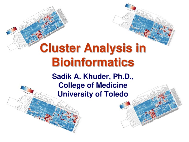
Cluster Analysis in Bioinformatics Sadik A. Khuder, Ph.D., College of Medicine University of Toledo

Cluster analysis Is the process of grouping several objects into a number of groups, or clusters. Objects in the same cluster are more similar to one another than they are to objects in other clusters.

What is clustering? A way of grouping together data samples that are similar in some way - according to some criteria that you pick A form of unsupervised learning you generally don t have examples demonstrating how the data should be grouped together It is a method of data exploration a way of looking for patterns or structure in the data that are of interest

What is a cluster? A cluster is a group that has homogeneity (internal cohesion) and separation (external isolation). The relationships between objects being studied are assessed by similarity or dissimilarity measures.

What is a cluster? Genome Biol 2010, 11:R124

The Goals of Clustering Identify patterns in the data Reduce complexity in data sets Allow visualization of complex data Data reduction natural clusters useful clusters outlier detection

The Need for Clustering Cluster variables (rows) Measure expression at multiple time-points, different conditions, etc. Similar expression patterns may suggest similar functions of genes

The Need for Clustering Cluster samples (columns) Expression levels of thousands of genes for each tumor sample Similar expression patterns may suggest biological relationship among samples Alizadeh et al., Nature 403:503-11, 2000

Similarity Measures The goal of cluster analysis is to group together similar data This depends on what we want to find or emphasize in the data The similarity measure is often more important than the clustering algorithm used The similarity measures are often replaced by dissimilarity measures

Distance Measures Given vectors x = (x1, , xn), y = (y1, , yn) Euclidean distance: n = i = 2) ( , ) ( d x y x y E i i 1 Manhattan distance: n 1 = i = ( , ) . d x y x y M i i

Euclidean distance deuc=0.5846 deuc=1.1345 deuc=1.41 deuc=2.6115 deuc=1.22

Correlation Coefficient The overall shape of expression profiles may be more important than the actual magnitudes Genes may be considered similar when they are up and down together The correlation coefficient may be more appropriate in these situations

Pearson Correlation Coefficient n = i ( )( ) x x y y i i = x y ( , ) 1 n n = i = i 2 2 ( ) ( ) x x y y i i 1 1 We re shifting the expression profiles down (subtracting the means) and scaling by the standard deviations (i.e., making the data have mean = 0 and std = 1)

Similarity: Jaccards coefficient Jaccard coefficient is used with binary data such as recording gene expression as on (1) or off (0) The coefficient (Sij) is defined as a = Sij + + a b c This is the ratio of positive matches to the total number of characters minus the number of negative matches. Genei 1 a 0 b Genej 1 0 c d

Clustering methods Partitioning Hierarchical

Hierarchical Method Hierarchical clustering Method produce a tree or dendogram They avoid specifying how many clusters are appropriate by providing a partition for each k obtained from cutting the tree at some level The tree can be built in two distinct ways Bottom-up: agglomerative clustering Top-down: divisive clustering

Dendogram A dendrogram shows how the clusters are merged hierarchically

Hierarchical Clustering Agglomerative Divisive Agglomerative clustering treats each object as a singleton cluster, and then successively merges clusters until all objects have been merged into a single remaining cluster. Divisive clustering works the other way around.

Agglomerative clustering 0 1 2 3 4 a a,b b c d e Kaufman and Rousseeuw (1990)

Agglomerative clustering 0 1 2 3 4 a a,b b c d d,e e Kaufman and Rousseeuw (1990)

Agglomerative clustering 0 1 2 3 4 a a,b b c c,d,e d d,e e Kaufman and Rousseeuw (1990)

Agglomerative clustering 0 1 2 3 4 a a,b b a,b,c,d,e c c,d,e d d,e e tree is constructed Kaufman and Rousseeuw (1990)

Divisive clustering a,b,c,d,e 4 3 2 1 0 Kaufman and Rousseeuw (1990)

Divisive clustering Divisive clustering a,b,c,d,e c,d,e 4 3 2 1 0 Kaufman and Rousseeuw (1990)

Divisive clustering Divisive clustering a,b,c,d,e c,d,e d,e 4 3 2 1 0 Kaufman and Rousseeuw (1990)

Divisive clustering Divisive clustering a,b a,b,c,d,e c,d,e d,e 4 3 2 1 0

Divisive clustering Divisive clustering a a,b b a,b,c,d,e c c,d,e d d,e e 4 3 0 2 1 tree is constructed Kaufman and Rousseeuw (1990)

Agglomerative Method Start with n sample clusters At each step, merge the two closet clusters using a measure of between-cluster dissimilarity which reflects the shape of the clusters The distance between clusters is defined by the method used

Cluster Linkage Methods Single linkage Complete linkage Centroid (Average linkage)

Example Single Linkage M T F A R N A 0 662 877 295 255 468 754 412 268 564 219 996 400 138 869 669 F M N R T A F M N R T 662 877 255 412 0 295 468 268 0 996 400 138 869 669 0 754 564 0 219 0

Example Single Linkage M T F A R N A 0 662 877 295 255 468 754 412 268 564 219 996 400 138 869 669 F M N R T A F M N R T 662 877 255 412 0 295 468 268 0 996 400 138 869 669 0 754 564 0 219 0

Example Single Linkage M T F A R N A 0 662 877 295 255 468 754 412 268 564 219 996 400 138 869 669 F M N R T A F M N R T 662 877 255 412 0 295 468 268 0 996 400 138 869 669 0 754 564 0 219 0

Example Single Linkage M T F A R N A 0 662 877 295 255 468 754 412 268 564 219 996 400 138 869 669 F M N R T A F M N R T 662 877 255 412 0 295 468 268 0 996 400 138 869 669 0 754 564 0 219 0

Example Single Linkage M T F A R N A 0 662 877 295 255 468 754 412 268 564 219 996 400 138 869 669 F M N R T A F M N R T 662 877 255 412 0 295 468 268 0 996 400 138 869 669 0 754 564 0 219 0

K-means clustering Step 0: Start with a random partition into K clusters Step 1: Generate a new partition by assigning each object to its closest cluster center Step 2: Compute new cluster centers as the centroids of the clusters. Reassign objects to the closest centroids. Step 3: Steps 1 and 2 are repeated until there is no change in the membership (also cluster centers remain the same)

K-means clustering 10 10 9 9 8 8 7 7 6 6 5 5 4 4 3 3 2 2 1 1 0 0 0 1 2 3 4 5 6 7 8 9 10 0 1 2 3 4 5 6 7 8 9 10 10 9 8 10 9 7 8 6 7 5 6 4 5 3 4 2 3 2 1 1 0 0 1 2 3 4 5 6 7 8 9 10 0 0 1 2 3 4 5 6 7 8 9 10

K-Means Method Strength Relatively efficient Often terminates at a local optimum. The global optimum may be found using techniques such as: deterministic annealing and genetic algorithms Weakness Applicable only when mean is defined Need to specify k, the number of clusters, in advance Unable to handle noisy data and outliers Not suitable to discover clusters with non-convex shapes

Determining the number of clusters We calculate a measure of cluster quality Q and then try different values of k until we get an optimal value for Q There are different choices of Q and our decision will depend on what dissimilarity measure we re using and what types of clusters we want Jagota suggests a measure that emphasizes cluster tightness or homogeneity: = i i C x x | | 1 1 k = x x ( , ) Q d i C i |Ci | is the number of data points in cluster I Q will be small if (on average) the data points in each cluster are close

Self-Organizing Maps (SOM) Based on work of Kohonen on learning/memory in the human brain As with k-means, we specify the number of clusters We also specify a topology a 2D grid that gives the geometric relationships between the clusters (i.e., which clusters should be near or distant from each other) The algorithm learns a mapping from the high dimensional space of the data points onto the points of the 2D grid (there is one grid point for each cluster)

Kohonen SOMs The Self-Organizing Map (SOM) is an unsupervised artificial neural network algorithm. It is a compromise between biological modeling and statistical data processing Each weight is representative of a certain input. Input patterns are shown to all neurons simultaneously. Competitive learning: the neuron with the largest response is chosen.

SOM

Kohonen SOMs Initialize weights Repeat until convergence Select next input pattern Find Best Matching Unit Update weights of winner and neighbours Decrease learning rate & neighbourhood size Learning rate & neighbourhood size

Example 1: clustering genes P. Tamayo et al., Interpreting patterns of gene expression with self-organizing maps: methods and application to hematopoietic differentiation, PNAS 96: 2907-12, 1999. Treatment of HL-60 cells (myeloid leukemia cell line) with PMA leads to differentiation into macrophages Measured expression of genes at 0, 0.5, 4 and 24 hours after PMA treatment

Example 1: clustering genes Used SOM technique; shown are cluster averages Clusters contain a number of known related genes involved in macrophage differentiation e.g., late induction cytokines, cell-cycle genes (down-regulated since PMA induces terminal differentiation), etc.

Example 2

Example 2 Single linkage Average linkage Complete linkage

Example 2

Example 2

Example 2

Example 2