Theory of Approximation: Interpolation
In the study of approximation theory, interpolation plays a crucial role in representing data points using polynomials and splines. This content discusses the concepts of interpolation polynomials, including Newton's Divided Difference and Lagrange Polynomials, as well as spline interpolation techniques such as linear, quadratic, and cubic splines. The focus is on fitting independent polynomials in intervals with continuity requirements, leading to a smoother representation of data. Various methods and conditions for spline interpolation are explored, providing insights into the mathematical foundations of approximation in data analysis.

Download Presentation

Please find below an Image/Link to download the presentation.
The content on the website is provided AS IS for your information and personal use only. It may not be sold, licensed, or shared on other websites without obtaining consent from the author.If you encounter any issues during the download, it is possible that the publisher has removed the file from their server.
You are allowed to download the files provided on this website for personal or commercial use, subject to the condition that they are used lawfully. All files are the property of their respective owners.
The content on the website is provided AS IS for your information and personal use only. It may not be sold, licensed, or shared on other websites without obtaining consent from the author.
E N D
Presentation Transcript
Theory of Approximation: Interpolation Abhas Singh Department of Civil Engineering IIT Kanpur Acknowledgements: Profs. Saumyen Guha and Shivam Tripathi (CE)
Interpolation Polynomials Newton s Divided Difference Lagrange Polynomials Direct Fit (Standard Format) Gram s polynomials (introduced earlier) Spline Interpolation: piecewise continuous, smoothing
Single Interpolation Polynomial If a single polynomial is fitted through a given set of points, the polynomial is always the same, irrespective of the basis used. Computation involved in obtaining the polynomial may vary depending on the basis. Since the polynomials are the same, the error in approximation may be obtained using the remainder term of the Newton s polynomial for all cases. So far, we have fitted one polynomial through all the n points. For a large number of points, this may lead to oscillations between the points, especially at the end intervals for the equally spaced data. Next we fit piecewise continuous polynomials or splines to the data!
Spline Interpolation Given: (n + 1) observations or data pairs [(x0, f0), (x1, f1), (x2, f2) (xn, fn)] This gives a mesh of nodes ?0,?1,?2, ?? on the independent variable and the corresponding function values as ?0,?1,?2, ?? Goal: fit an independent polynomial in each interval (between two points) with certain continuity requirements at the nodes. Linear spline: continuity in function values, C0 continuity Quadratic spline: continuity in function values and 1st derivatives, C1 continuity Cubic spline: continuity in function values, 1st and 2nd derivatives, C2 continuity Denote for node i or at xi: functional value fi, first derivative ui, second derivative vi
Spline Interpolation: Linear xi+2, fi+2 xi, fi qi+1(x) qi(x) qi(xi) = fi qi-1(xi) = qi(xi) xi+1, fi+1 qi-1(x) xi-1, fi-1 A straight line in each interval: (n+1) points, n straight lines, 2n unknowns Available conditions: (n+1) function values, (n-1) function continuity conditions Straight lines can be uniquely estimated!
Spline Interpolation: Linear Let us denote the Linear Spline in the interval ??,??+1 as ??? We know: ???? = ? ?? = ?? and ????+1 = ? ??+1 = ??+1 Therefore, the Linear Spline in the interval ??,??+1: ? ??+1 ?? ??+1+ ??+1 ? ?? ??+1 ??, using the Lagrange polynomial ??? = ?? Let us denote the length of the ith interval ??,??+1 as ?= ??+1 ?? The linear spline at the ith interval is then given by: ??? =??+1 ? ?? ?? ? ????? ? ??+1 = ? ??+1,?? ? ?? + ?? ? ? ? ? ?? ?? ?? q ? = ?=0 ??? = ?=0 ? ?
Spline Interpolation: Quadratic xi+2, fi+2 xi, fi qi(x) qi+1(x) xi+1, fi+1 qi-1(x) xi-1, fi-1 ???? = ?? ?? 1?? = ???? ?? 1 ?? = ??= ?? ?? A quadratic polynomial in each interval: (n+1) points, n quadratic polynomials, 3n unknowns Available conditions: (n + 1) function values, (n - 1) function continuity and (n - 1) 1st derivative continuity conditions, total 3n-1 conditions. 1 free condition to be chosen by the user!
Spline Interpolation: Quadratic Quadratic Spline in the interval ??,??+1: ??? ?? Let us denote the derivative (u) of the function at the ith node as ? ?? = ? ?? = ?? Therefore: ?? We may write: ? =??+1 ? ??? =??+1 2 ? ? is a set of linear splines. ?? = ? ?? = ?? and ?? ??+1 = ? ??+1 = ??+1 ? ?? ?? ?? ? ??+1 ? ?? 2 ? 2 2+ ? ? ?? ? ??+1 ? = ??+?? ? ??+1= 2? ??+1,?? ?? ???? = ?? 2 ????+1 = ??+1 Recall one free condition, either u0 or un is specified!
Spline Interpolation: Cubic xi+2, fi+2 xi, fi qi(x) qi+1(x) xi+1, fi+1 qi-1(x) ???? = ?? ?? 1?? = ???? ?? 1 ?? = ??= ?? ?? 1 ?? = ??= ?? xi-1, fi-1 ?? ?? A cubic polynomial in each interval: (n+1) points, n cubic polynomials, 4n unknowns Available conditions: (n + 1) function values, (n - 1) function continuity, (n - 1) 1st derivative continuity conditions and (n - 1) 2nd derivative continuity conditions, total 4n - 2 conditions. 2 free conditions to be chosen by the user!
Spline Interpolation: Cubic Cubic Spline in the interval ??,??+1: ??? ?? Let us denote the 2nd derivative (v) of the function at the ith node as ? ?? = ? ?? = ?? Therefore: ?? We may write: ? =??+1 ? ??? =??+1 6 ? ???? = ??=?? ? ? is a set of linear splines. ?? = ? ?? = ?? and ?? ??+1 = ? ??+1 = ??+1 ? ?? ?? ?? 6 ? ?? ? ??+1 ? 3 3+ ?1? + ?2 ? ?? ? ??+1 2 + ?1??+ ?2 2 + ?1??+1+ ?2 6 ????+1 = ??+1=??+1 ? 6
Spline Interpolation: Cubic ??? =??+1 ?? 6 ? 3 3+ ?1? + ?2 ? ?? ? ??+1 6 ? 2 2 ???? = ??=?? ? ?1= ? ??+1,?? ? ????+1 = ??+1=??+1 ? ??+1 ?? =??+1 ? ??+?? ? + ?1??+ ?2; + ?1??+1+ ?2 6?? ? 6 6 ?? + ? 6??+1 6 ? ?2= ??+1 ??+1 ? 6????+1+ ? 6??+1?? ? ??? =??+1 3 3 ? ?? ? ? ?? ?? +?? ? ??+1 ? ?? ?? + ?? ??+1 6 6 +??+1 ? ??+1 ? ? We need to estimate (n + 1) unknown vi. We have (n 1) conditions from the continuity of the first derivative.
Spline Interpolation: Cubic ?? = ?? 1 ?? ??; ? = 1,2,3, ? 1 (??.1) ??? =??+1 3 3 ? ?? ? +?? ? ??+1 ? ? +?? +??+1 ? ?? ?? ?? ?? + ?? ??+1 ? ??+1 6 6 ? ? 2 2 ? =??+1 3 ? ?? 3 ? ??+1 ?? + ? + ? ??+1,?? 6 ? 6 ? 2 2 ? =?? 3 ? ?? 1 ? 1 ? 1 +?? 1 3 ? ?? ?? 1 + ? 1 + ? ??,?? 1 6 6 ? 1 In eq. (1), 6??+1 ? ? 1 6 ?? ? ? ? 3??+ ? ??+1,?? = ? 1 ?+ ? 1 3 ??+ ?? ? ? ??+ ? 1 ?? 1+ ? ??,?? 1 3 6 ?? ? ?? 1 6??+1= ? ??,?? 1 ? ??+1,?? ??+?? ???+?= ? ??+?,?? ? ??,?? ? ?? ?+ ?? ??? ?+ ? ??+ ?? ???+ ????+?= ?? ??+?,?? ?? ??,?? ?
Spline Interpolation: Cubic ?? ??? ?+ ? ??+ ?? ???+ ????+?= ?? ??+?,?? ?? ??,?? ? ? = 1,2,3, ? 1. So, (n 1) equations, (n + 1) unknowns, two conditions have to be provided by the users. They decide the type of cubic splines Natural Spline: ?0= ??= 0 Parabolic Runout: ?0= ?1 and Not-a-knot: ?? 1= ?? ?1 ?0 0 ?? 1 ?? 2 ? 2 =?2 ?1 ?0? = ?1? 1 =?? ?? 1 ? 1 ?? 2? = ?? 1? Periodic: ?0= ??; ?0= ?? and ?0= ?? First one comes from the data (if not satisfied, the periodic spline is not appropriate); the next two give the other two equations.
Spline Interpolation: Cubic ?? ??? ?+ ? ??+ ?? ???+ ????+?= ?? ??+?,?? ?? ??,?? ? ? = 1,2,3, ? 1. So, (n 1) equations, (n + 1) unknowns, two conditions have to be provided by the users. They decide the type of cubic splines Clamped Spline: ?0 = ? 3 ? ?0 0 ?0 0 3 3 ? ?? 1 ? 1 ?? =?? ? 1 ?0= ?0 and ??= ?? 1 3 ? ?1 0 ?? = 2 2 ? =?1 0 +?0 ?0 + 0 + ? ?1,?0 6 6 ?0 = ?1 0 ? ?? ?0 + ? ?1,?0 = ? ???+ ??= ? ??,?? ? 6 2 2 ? =?? ? 1 +?? 1 3 ? ?? ? 1 ?? 1 + ? 1 + ? ??,?? 1 6 6 +?? 1 ? 1 ?? 1 + ? ??,?? 1 = 3 6 ? ???+ ?? ?= ? ? ??,?? ? ?? ?
Example Problem: Q4 of Tutorial 9 Consider the function sampled at points = 0 0.5, 1.0, 1.5 and 2 , x Estimate the function value at x = 1.80 by interpolating the function using - (a) natural cubic spline and (b) not-a-knot cubic spline. Calculate the true percentage error for both the splines. Which is the better spline for this problem and why? Solution: Posted online along with Tutorial 9 solutions