The Ups and Downs of Backpropagation in Neural Networks
The history and failure of backpropagation in the 1990s are discussed, highlighting its potential and limitations. The challenges faced due to slow computers, small datasets, and network architecture are explained. The comparison with Support Vector Machines for Artificial Intelligence tasks is explored along with various machine learning task scenarios.

Download Presentation

Please find below an Image/Link to download the presentation.
The content on the website is provided AS IS for your information and personal use only. It may not be sold, licensed, or shared on other websites without obtaining consent from the author.If you encounter any issues during the download, it is possible that the publisher has removed the file from their server.
You are allowed to download the files provided on this website for personal or commercial use, subject to the condition that they are used lawfully. All files are the property of their respective owners.
The content on the website is provided AS IS for your information and personal use only. It may not be sold, licensed, or shared on other websites without obtaining consent from the author.
E N D
Presentation Transcript
Neural Networks for Machine Learning Lecture 13a The ups and downs of backpropagation Geoffrey Hinton Nitish Srivastava, Kevin Swersky Tijmen Tieleman Abdel-rahman Mohamed
A brief history of backpropagation The backpropagation algorithm for learning multiple layers of features was invented several times in the 70 s and 80 s: Bryson & Ho (1969) linear Werbos (1974) Rumelhart et. al. in 1981 Parker (1985) LeCun (1985) Rumelhart et. al. (1985) Backpropagation clearly had great promise for learning multiple layers of non-linear feature detectors. But by the late 1990 s most serious researchers in machine learning had given up on it. It was still widely used in psychological models and in practical applications such as credit card fraud detection.
Why backpropagation failed The popular explanation of why backpropagation failed in the 90 s: It could not make good use of multiple hidden layers. (except in convolutional nets) It did not work well in recurrent networks or deep auto-encoders. Support Vector Machines worked better, required less expertise, produced repeatable results, and had much fancier theory. The real reasons it failed: Computers were thousands of times too slow. Labeled datasets were hundreds of times too small. Deep networks were too small and not initialized sensibly. These issues prevented it from being successful for tasks where it would eventually be a big win.
A spectrum of machine learning tasks Typical Statistics---------------Artificial Intelligence Low-dimensional data (e.g. less than 100 dimensions) Lots of noise in the data. Not much structure in the data. The structure can be captured by a fairly simple model. The main problem is separating true structure from noise. Not ideal for non-Bayesian neural nets. Try SVM or GP. High-dimensional data (e.g. more than 100 dimensions) The noise is not the main problem. There is a huge amount of structure in the data, but its too complicated to be represented by a simple model. The main problem is figuring out a way to represent the complicated structure so that it can be learned. Let backpropagation figure it out.
Why Support Vector Machines were never a good bet for Artificial Intelligence tasks that need good representations View 1: SVM s are just a clever reincarnation of Perceptrons. They expand the input to a (very large) layer of non- linear non-adaptive features. They only have one layer of adaptive weights. They have a very efficient way of fitting the weights that controls overfitting. View 2: SVM s are just a clever reincarnation of Perceptrons. They use each input vector in the training set to define a non-adaptive pheature . The global match between a test input and that training input. They have a clever way of simultaneously doing feature selection and finding weights on the remaining features.
Historical document from AT&T Adaptive Systems Research Dept., Bell Labs
Neural Networks for Machine Learning Lecture 13b Belief Nets Geoffrey Hinton Nitish Srivastava, Kevin Swersky Tijmen Tieleman Abdel-rahman Mohamed
What is wrong with back-propagation? It requires labeled training data. Almost all data is unlabeled. The learning time does not scale well It is very slow in networks with multiple hidden layers. Why? It can get stuck in poor local optima. These are often quite good, but for deep nets they are far from optimal. Should we retreat to models that allow convex optimization?
Overcoming the limitations of back-propagation by using unsupervised learning The learning objective for a generative model: Maximise p(x) not p(y | x) What kind of generative model should we learn? An energy-based model like a Boltzmann machine? A causal model made of idealized neurons? A hybrid of the two? Keep the efficiency and simplicity of using a gradient method for adjusting the weights, but use it for modeling the structure of the sensory input. Adjust the weights to maximize the probability that a generative model would have generated the sensory input. If you want to do computer vision, first learn computer graphics.
Artificial Intelligence and Probability Many ancient Greeks supported Socrates opinion that deep, inexplicable thoughts came from the gods. Today s equivalent to those gods is the erratic, even probabilistic neuron. It is more likely that increased randomness of neural behavior is the problem of the epileptic and the drunk, not the advantage of the brilliant. P.H. Winston, Artificial Intelligence , 1977. (The first AI textbook) All of this will lead to theories of computation which are much less rigidly of an all-or-none nature than past and present formal logic ... There are numerous indications to make us believe that this new system of formal logic will move closer to another discipline which has been little linked in the past with logic. This is thermodynamics primarily in the form it was received from Boltzmann. John von Neumann, The Computer and the Brain , 1958 (unfinished manuscript)
The marriage of graph theory and probability theory Graphical models: Pearl, Heckerman, Lauritzen, and many others showed that probabilities worked better. Graphs were good for representing what depended on what. Probabilities then had to be computed for nodes of the graph, given the states of other nodes. Belief Nets: For sparsely connected, directed acyclic graphs, clever inference algorithms were discovered. In the 1980 s there was a lot of work in AI that used bags of rules for tasks such as medical diagnosis and exploration for minerals. For practical problems, they had to deal with uncertainty. They made up ways of doing this that did not involve probabilities!
Belief Nets A belief net is a directed acyclic graph composed of stochastic variables. We get to observe some of the variables and we would like to solve two problems: The inference problem: Infer the states of the unobserved variables. The learning problem: Adjust the interactions between variables to make the network more likely to generate the training data. stochastic hidden causes visible effects
Graphical Models versus Neural Networks Early graphical models used experts to define the graph structure and the conditional probabilities. The graphs were sparsely connected. Researchers initially focused on doing correct inference, not on learning. For neural nets, learning was central. Hand-wiring the knowledge was not cool (OK, maybe a little bit). Knowledge came from learning the training data. Neural networks did not aim for interpretability or sparse connectivity to make inference easy. Nevertheless, there are neural network versions of belief nets.
Two types of generative neural network composed of stochastic binary neurons Causal: We connect binary stochastic neurons in a directed acyclic graph to get a Sigmoid Belief Net (Neal 1992). Energy-based: We connect binary stochastic neurons using symmetric connections to get a Boltzmann Machine. If we restrict the connectivity in a special way, it is easy to learn a Boltzmann machine. But then we only have one hidden layer. stochastic hidden causes visible effects
Neural Networks for Machine Learning Lecture 13c Learning Sigmoid Belief Nets Geoffrey Hinton Nitish Srivastava, Kevin Swersky Tijmen Tieleman Abdel-rahman Mohamed
Learning Sigmoid Belief Nets It is easy to generate an unbiased example at the leaf nodes, so we can see what kinds of data the network believes in. It is hard to infer the posterior distribution over all possible configurations of hidden causes. It is hard to even get a sample from the posterior. So how can we learn sigmoid belief nets that have millions of parameters? stochastic hidden causes visible effects
The learning rule for sigmoid belief nets Learning is easy if we can get an unbiased sample from the posterior distribution over hidden states given the observed data. j j s w ji i s i For each unit, maximize the log prob. that its binary state in the sample from the posterior would be generated by the sampled binary states of its parents. 1 pi p(si=1)= j 1+exp -bi- sjwji) ( = ) w s s p ji j i i
Explaining away (Judea Pearl) Even if two hidden causes are independent in the prior, they can become dependent when we observe an effect that they can both influence. If we learn that there was an earthquake it reduces the probability that the house jumped because of a truck. -10 -10 posterior over hiddens truck hits house earthquake p(1,1)=.0001 p(1,0)=.4999 p(0,1)=.4999 p(0,0)=.0001 20 20 -20 house jumps
Why its hard to learn sigmoid belief nets one layer at a time To learn W, we need to sample from the posterior distribution in the first hidden layer. Problem 1: The posterior is not factorial because of explaining away . Problem 2: The posterior depends on the prior as well as the likelihood. So to learn W, we need to know the weights in higher layers, even if we are only approximating the posterior. All the weights interact. Problem 3: We need to integrate over all possible configurations in the higher layers to get the prior for first hidden layer. Its hopeless! hidden variables hidden variables prior hidden variables W data
Some methods for learning deep belief nets Monte Carlo methods can be used to sample from the posterior (Neal 1992). But its painfully slow for large, deep belief nets. In the 1990 s people developed variational methods for learning deep belief nets. These only get approximate samples from the posterior. Learning with samples from the wrong distribution: Maximum likelihood learning requires unbiased samples from the posterior. What happens if we sample from the wrong distribution but still use the maximum likelihood learning rule? Does the learning still work or does it do crazy things?
Neural Networks for Machine Learning Lecture 13d The wake-sleep algorithm Geoffrey Hinton Nitish Srivastava, Kevin Swersky Tijmen Tieleman Abdel-rahman Mohamed
An apparently crazy idea Crazy idea: do the inference wrong. Maybe learning will still work. This turns out to be true for SBNs. At each hidden layer, we assume (wrongly) that the posterior over hidden configurations factorizes into a product of distributions for each separate hidden unit. It s hard to learn complicated models like Sigmoid Belief Nets. The problem is that it s hard to infer the posterior distribution over hidden configurations when given a datavector. Its hard even to get a sample from the posterior.
Factorial distributions In a factorial distribution, the probability of a whole vector is just the product of the probabilities of its individual terms: individual probabilities of three hidden units in a layer 0.3 0.6 0.8 probability that the hidden units have state 1,0,1 if the distribution is factorial. p(1, 0,1)=0.3 (1-0.6) 0.8 A general distribution over binary vectors of length N has 2^N degrees of freedom (actually 2^N-1 because the probabilities must add to 1). A factorial distribution only has N degrees of freedom.
The wake-sleep algorithm (Hinton et. al. 1995) Wake phase: Use recognition weights to perform a bottom-up pass. Train the generative weights to reconstruct activities in each layer from the layer above. h3 W3 R3 h2 W2 R2 Sleep phase: Use generative weights to generate samples from the model. Train the recognition weights to reconstruct activities in each layer from the layer below. h1 R1 W1 data
The flaws in the wake-sleep algorithm The recognition weights are trained to invert the generative model in parts of the space where there is no data. This is wasteful. The recognition weights do not follow the gradient of the log probability of the data. They only approximately follow the gradient of the variational bound on this probability. This leads to incorrect mode-averaging The posterior over the top hidden layer is very far from independent because of explaining away effects. Nevertheless, Karl Friston thinks this is how the brain works.
Mode averaging If we generate from the model, half the instances of a 1 at the data layer will be caused by a (1,0) at the hidden layer and half will be caused by a (0,1). So the recognition weights will learn to produce (0.5, 0.5) This represents a distribution that puts half its mass on 1,1 or 0,0: very improbable hidden configurations. Its much better to just pick one mode. This is the best recognition model you can get if you assume that the posterior over hidden states factorizes. -10 -10 ? ? +20 +20 -20 1 a better solution mode averaging true bimodal posterior


")


")