The Basics of t-Test in Social Statistics
What is t test
Types of t test
TTEST function
T-test ToolPak
2
In most cases, the z-test requires more information
than we have available
We do inferential statistics to learn about the
unknown population but, ironically, we need to know
characteristics of the population to make inferences
about it
Enter the t-test: “estimate what you don’t know”
3
Employed by Guinness Brewery,
Dublin, Ireland, from 1899 to
1935.
Developed t-test around 1905, for
dealing with small samples in
brewing quality control.
Published in 1908 under
pseudonym “Student” (“Student’s
t-test”)
4
5
Degrees of freedom describes the number of
scores in a sample that are free to vary.
degrees of freedom = df = n-1
The larger, the better
6
Very similar like z test
Use sample statistics instead of population
parameters (mean and standard deviation)
Evaluate the result through t test table instead
of z test table
7
We show 26 babies the two pictures at the same time (one
with his/her mother, the other a scenery picture) for 60
seconds, and measure how long they look at the facial
configuration.
Our null assumption is that they will not look at it for longer
than half the time, μ = 30
Our alternate hypothesis is that they will look at the face
stimulus longer and face recognition is hardwired in their
brain, not learned (directional)
Our sample of n = 26 babies looks at the face stimulus for M =
35 seconds, s = 16 seconds
Test our hypotheses (α = .05, one-tailed)
8
Sentence:
Null: Babies look at the face stimulus for less than
or equal to half the time
Alternate: Babies look at the face stimulus for
more than half the time
Code Symbols:
9
Population variance is not known, so use
sample variance to estimate
n = 26 babies; df = n-1 = 25
Look up values for t at the limits of the critical
region from our critical values of t table
Set α = .05; one-tailed
tcrit = +1.708
10
Central Limit Theorem
μ = 30
s
M
=s/ =16/ = 3.14
11
The tobt=1.59 does not exceed tcrit=1.708
∴
We must retain the null hypothesis
Conclusion: Babies do not look at the face
stimulus more often than chance, t(25) =
+1.59, n.s., one-tailed. Our results do not
support the hypothesis that face processing is
innate.
12
A research design that uses a separate sample
for each treatment condition is called an
independent-measures (or between-subjects)
research design.
13
The goal of an independent-measures research
study:
To evaluate the difference of the means between
two populations.
Mean of first population: μ1
Mean of second population: μ2
Difference between the means: μ1- μ2
14
Null hypothesis: “no change = no effect = no
difference”
H0: μ1- μ2 = 0
Alternative hypothesis: “there is a difference”
H1: μ1- μ2 ≠ 0
15
Value for degrees of freedom: df = df1 + df2
16
17
Step 1: A statement of the null and research
hypotheses.
Null hypothesis: there is no difference between
two groups
Research hypothesis: there is a difference between
the two groups
18
Step 2: setting the level of risk (or the level of
significance or Type I error) associated with
the null hypothesis
0.05
19
Step 3: Selection of the appropriate test
statistic
Determine which test statistic is good for your
research
Independent t test
20
Step 4: computation of the test statistic value
t= 0.14
21
Step 5: determination of the value needed for
the rejection of the null hypothesis
T Distribution Critical Values Table
22
Step 5
: (cont.)
Degrees of freedom (df): approximates the sample size
Group 1 sample size -1 + group 2 sample size -1
Our test df = 58
Two-tailed or one-tailed
Directed research hypothesis
one-tailed
Non-directed research hypothesis
two-tailed
23
Step 6: A comparison of the obtained value
and the critical value
0.14 and 2.001
If the obtained value > the critical value, reject the
null hypothesis
If the obtained value < the critical value, retain the
null hypothesis
24
Step 7 and 8: make a decision
What is your decision and why?
25
How to interpret t
(58)
= 0.14, p>0.05, n.s.
26
T.TEST (array1, array2, tails, type)
array1 = the cell address for the first set of data
array2 = the cell address for the second set of
data
tails: 1 = one-tailed, 2 = two-tailed
type: 1 = a paired t test;
2 = a two-sample test
(independent with equal variances)
; 3 = a
two-sample test with unequal variances
27
It does not compute the t value
It returns the likelihood that the resulting t
value is due to chance (the possibility of the
difference of two groups is due to chance)
28
Select
t-Test: Two-Sample Assuming Equal Variances
29
If two groups are different, how to measure
the difference among them
Effect size
ES: effect size
: the mean for Group 1
: the mean for Group 2
SD: the standard deviation from either group
30
A small effect size ranges from 0.0 ~ 0.2
Both groups tend to be very similar and overlap a lot
A medium effect size ranges from 0.2 ~ 0.5
The two groups are different
A large effect size is any value above 0.50
The two groups are quite different
ES=0
the two groups have no difference and overlap entirely
ES=1
the two groups overlap about 45%
31
Explore the significance of the t-test for inferential statistics, its types, and why it is preferred over the z-test in many cases. Learn about William S. Gossett's contribution to the development of the t-test and understand concepts like degrees of freedom. Delve into practical applications with a detailed example involving hypothesis testing for babies' face stimulus recognition.

Download Presentation

Please find below an Image/Link to download the presentation.
The content on the website is provided AS IS for your information and personal use only. It may not be sold, licensed, or shared on other websites without obtaining consent from the author.If you encounter any issues during the download, it is possible that the publisher has removed the file from their server.
You are allowed to download the files provided on this website for personal or commercial use, subject to the condition that they are used lawfully. All files are the property of their respective owners.
The content on the website is provided AS IS for your information and personal use only. It may not be sold, licensed, or shared on other websites without obtaining consent from the author.
E N D
Presentation Transcript
This week What is t test Types of t test TTEST function T-test ToolPak 2
Why not z-test In most cases, the z-test requires more information than we have available We do inferential statistics to learn about the unknown population but, ironically, we need to know characteristics of the population to make inferences about it Enter the t-test: estimate what you don t know 3
William S. Gossett Employed by Guinness Brewery, Dublin, Ireland, from 1899 to 1935. Developed t-test around 1905, for dealing with small samples in brewing quality control. Published in 1908 under pseudonym Student ( Student s t-test ) 4
Degrees of Freedom and t test Degrees of freedom describes the number of scores in a sample that are free to vary. degrees of freedom = df = n-1 The larger, the better 6
One sample t test Very similar like z test Use sample statistics instead of population parameters (mean and standard deviation) Evaluate the result through t test table instead of z test table 7
An example We show 26 babies the two pictures at the same time (one with his/her mother, the other a scenery picture) for 60 seconds, and measure how long they look at the facial configuration. Our null assumption is that they will not look at it for longer than half the time, = 30 Our alternate hypothesis is that they will look at the face stimulus longer and face recognition is hardwired in their brain, not learned (directional) Our sample of n = 26 babies looks at the face stimulus for M = 35 seconds, s = 16 seconds Test our hypotheses ( = .05, one-tailed) 8
Step 1: Hypotheses Sentence: Null: Babies look at the face stimulus for less than or equal to half the time Alternate: Babies look at the face stimulus for more than half the time Code Symbols: 9
Step 2: Determine Critical Region Population variance is not known, so use sample variance to estimate n = 26 babies; df = n-1 = 25 Look up values for t at the limits of the critical region from our critical values of t table Set = .05; one-tailed tcrit = +1.708 10
Step 3: Calculate t statistic from sample Central Limit Theorem = 30 sM=s/ =16/ = 3.14 n 26 11
Step 4: Decision and Conclusion The tobt=1.59 does not exceed tcrit=1.708 We must retain the null hypothesis Conclusion: Babies do not look at the face stimulus more often than chance, t(25) = +1.59, n.s., one-tailed. Our results do not support the hypothesis that face processing is innate. 12
Independent t test A research design that uses a separate sample for each treatment condition is called an independent-measures (or between-subjects) research design. 13
t Statistic for Independent- Measures Design The goal of an independent-measures research study: To evaluate the difference of the means between two populations. Mean of first population: 1 Mean of second population: 2 Difference between the means: 1- 2 14
t Statistic for Independent- Measures Design Null hypothesis: no change = no effect = no difference H0: 1- 2 = 0 Alternative hypothesis: there is a difference H1: 1- 2 0 15
T test formula x x = 1 n 2 t + n + n 2 1 2 2 ( ) 1 n ( ) 1 n s s n n 1 2 1 n 2 + 2 1 2 1 2 ?1: is the mean for Group 1 ?2: is the mean for Group 2 ?1: is the number of participants in Group 1 ?2: is the number of participants in Group 2 ?12: is the variance for Group 1 ?22: is the variance for Group 20 Value for degrees of freedom: df = df1 + df2 16
An Example Group 1 Group 2 7 3 3 2 3 8 8 5 8 5 5 4 6 5 7 1 9 2 5 2 5 4 4 5 5 7 8 8 9 8 3 2 5 4 4 6 7 7 5 6 4 3 2 7 6 2 8 9 7 6 10 10 5 1 1 4 3 12 15 4 17
T test steps Step 1: A statement of the null and research hypotheses. Null hypothesis: there is no difference between two groups 0: = H 1 2 Research hypothesis: there is a difference between the two groups 1: H 1 2 18
T test steps Step 2: setting the level of risk (or the level of significance or Type I error) associated with the null hypothesis 0.05 19
T test steps Step 3: Selection of the appropriate test statistic Determine which test statistic is good for your research Independent t test 20
T test steps Step 4: computation of the test statistic value t= 0.14 21
T test steps Step 5: determination of the value needed for the rejection of the null hypothesis T Distribution Critical Values Table 22
T test steps Step 5: (cont.) Degrees of freedom (df): approximates the sample size Group 1 sample size -1 + group 2 sample size -1 Our test df = 58 Two-tailed or one-tailed Directed research hypothesis one-tailed Non-directed research hypothesis two-tailed 23
T test steps Step 6: A comparison of the obtained value and the critical value 0.14 and 2.001 If the obtained value > the critical value, reject the null hypothesis If the obtained value < the critical value, retain the null hypothesis 24
T test steps Step 7 and 8: make a decision What is your decision and why? 25
Interpretation How to interpret t(58) = 0.14, p>0.05, n.s. 26
Excel: T.TEST function T.TEST (array1, array2, tails, type) array1 = the cell address for the first set of data array2 = the cell address for the second set of data tails: 1 = one-tailed, 2 = two-tailed type: 1 = a paired t test; 2 = a two-sample test (independent with equal variances); 3 = a two-sample test with unequal variances 27
Excel: T.TEST function It does not compute the t value It returns the likelihood that the resulting t value is due to chance (the possibility of the difference of two groups is due to chance) 28
Excel ToolPak Select t-Test: Two-Sample Assuming Equal Variances t-Test: Two-Sample Assuming Equal Variances Variable 1 5.433333333 11.70229885 Variable 2 5.533333333 4.257471264 Mean Variance Observations Pooled Variance Hypothesized Mean Difference df t Stat P(T<=t) one-tail t Critical one-tail P(T<=t) two-tail t Critical two-tail 30 30 7.979885057 0 58 -0.137103112 0.44571206 1.671552763 0.891424121 2.001717468 29
Effect size If two groups are different, how to measure the difference among them Effect size 1 X X = 2 ES SD ES: effect size : the mean for Group 1 : the mean for Group 2 SD: the standard deviation from either group X X 1 2 30
Effect size A small effect size ranges from 0.0 ~ 0.2 Both groups tend to be very similar and overlap a lot A medium effect size ranges from 0.2 ~ 0.5 The two groups are different A large effect size is any value above 0.50 The two groups are quite different ES=0 the two groups have no difference and overlap entirely ES=1 the two groups overlap about 45% 31