System Transfer Functions
Learn about transfer functions in system analysis, how to obtain them through Laplace transforms, characteristic equations, poles, and zeros. Explore the relationship between input and output in a system.

Download Presentation

Please find below an Image/Link to download the presentation.
The content on the website is provided AS IS for your information and personal use only. It may not be sold, licensed, or shared on other websites without obtaining consent from the author.If you encounter any issues during the download, it is possible that the publisher has removed the file from their server.
You are allowed to download the files provided on this website for personal or commercial use, subject to the condition that they are used lawfully. All files are the property of their respective owners.
The content on the website is provided AS IS for your information and personal use only. It may not be sold, licensed, or shared on other websites without obtaining consent from the author.
E N D
Presentation Transcript
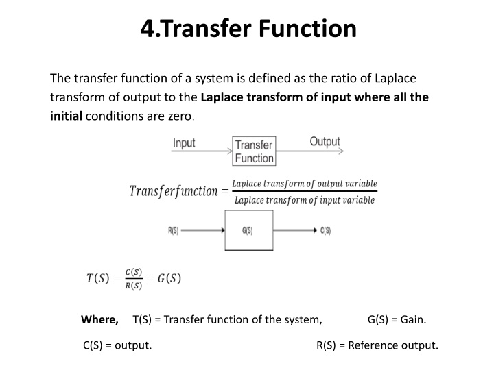
4.Transfer Function The transfer function of a system is defined as the ratio of Laplace transform of output to the Laplace transform of input where all the initial conditions are zero. Where, T(S) = Transfer function of the system, G(S) = Gain. C(S) = output. R(S) = Reference output.
4.1 Steps to obtain transfer function - Step-1 Write the differential equation. Step-2 Find out Laplace transform of the equation assuming 'zero' as an initial condition. Step-3 Take the ratio of output to input. Step-4 Write down the equation of G(S) as follows - Here, a and b are constants, and S is a complex variable
4.1 Characteristic equation of a transfer function - Here, the characteristic equation of a linear system can be obtained by equating the denominator polynomial of a transfer function is zero. Thus the characteristic equation of the transfer function of Eq.1 will be: ansn+a(n-1)s(n-1)+.........+a1s+a0=0 4.2 Poles and Zeros of a transfer function - and n terms respectively: Consider the equation 1, the numerator and denominator can be factored in m K = Dm / an is known as the gain factor and's' is the complex frequency. Where,
Poles: Poles are the frequencies of the transfer function for which the value of the transfer function becomes infinity. Zeros: Zeros are the frequencies of the transfer function for which the value of the transfer function becomes zero. polynomial (poles and zeros) We will apply the following standard equation to find the roots of multiple poles or multiple zeros. If any poles or zeros coincide then such poles and zeros are called called simple poles or simple zeros. If the poles and zeros do not coincide then such poles and zeros are
For example- S = -2, and multiple poles at S = -4 i.e. the pole of order 2 at S = -4. The zeros of the function are S = -3 and the poles of the function are S = 0, The two cases that arise when we consider the whole 'S' plane is: transfer function becomes infinity for S = -p and the order of such poles is P-Z. 1. If the no. of zeros are less than no. of poles, i.e., Z<P then the value of transfer function becomes zero for S = -Z , and the order of such zeross is Z-P. 2. If the no. of poles are less than no. of zeros P<Z then the value of The symbols that are used to locate poles and zeros on S-plane are X and O . The pole is represented by X and zero is represented by O . The pole-zero plot of the above example is as follows -
Step 2: By taking the Laplace transform of eq (1) and eq (2) and assuming all initial condition to be zero. Step 3: Calculation of transfer function Eq (5) is the transfer function
5.3 How to draw the block Diagram: Consider a simple R-L circuit Applying KCL Now taking Laplace transform of Eq.1 and Eq.2 with initial condition zero From fig.: For the right-hand side of eq.5, we will use a summing point.
Here the output of summing point is given to the block, and the output of the block is I(s) Now the output I(s) is given to another block containing element SL and the output of this block is V0. By combining the above two figures, we get the required block diagram.
Closed loop control system A system in which there is a feedback path is called a closed-loop control system. In this system, the output is feedback into the error detector and then it is compared with the input signal. The feedback signal can be negative or positive. For posative Feedback For negative Feedback
5.4 Block diagram reduction rules Rule No.1. Blocks in Cascade When two or more blocks are connected in series, then the resultant block is the product of the individual blocks. Rule No.2 Blocks in parallel When two or more blocks are connected in parallel, then the resultant block is the sum of the individual blocks.
Rule No.3 Moving a take-off point ahead of a block When the take-off point is moved ahead of a block (before the block), then the same transfer function is introduced in the take-off point branch. Rule No.4 Moving the take-off point after the block When the take-off point is moved after the block, then a block with reciprocal of a transfer function is introduced in the take-off point branch.
Rule No.5 Moving a summing point beyond the block Rule No.6:Moving a summing point ahead of a block Rule No.7:Eliminating a forward loop
Example 5-1 Find the transfer function of the following by block reduction technique. Solution Step 1: There are two internal closed loops. Firstly, we will remove this loop. Step 2: When the two blocks are in a cascade or series we will use rule no.1. Step 3: Now we will solve this loop.
loop containing H1, we obtain EXAMPLE Consider the system shown in Figure , Simplify this diagram. By moving the summing point of the negative feedback loop containing H2 outside the positive feedback Eliminating the positive feedback loop. The elimination of the loop containing H2/G1 gives Figure(d).


 and")
")