Seldom Taught Statistical Techniques
Some simple, useful, but
seldom taught statistical
techniques
Larry Weldon
Statistics and Actuarial Science
Simon Fraser University
Nov. 27, 2008
1
Outline of Talk
•
Why simple techniques overlooked
•
Simplest kernel estimation and smoothing
•
Simplest multivariate data display
•
Simplest bootstrap
•
Expanded use of Simulation
•
Conclusion
Some simple, useful, but seldom taught statistical techniques
Evolution of Good Ideas in Stats
•
New idea proposed by researcher
(e.g. Loess smoothing, bootstrap, coplots)
•
Developed by researchers to optimal form
(usually mathematically complex)
•
Considered too advanced for undergrad
•
Undergrad courses do not include good
ideas
What new techniques can
undergrad stats use?
•
Simplest kernel estimation and smoothing
•
Simplest multivariate data display
•
Simplest bootstrap
•
Expanded use of Simulation
What new techniques can
undergrad stats use?
•
Simplest kernel estimation and smoothing
•
Simplest multivariate data display
•
Simplest bootstrap
•
Expanded use of Simulation
Kernel Estimation
Windowgrams and
Non-Parametric Smoothers
Histogram
Primitive “Windowgram”
Estimate density at grid points
9
d
Windowgram
•
Just records frequency withing “d” of grid
point.
•
Like using rectangular “window”
0
1
Grid point
Weight Function
d
Primitive “Windowgram”
go to R
Count at grid
Join grid counts
Rescale to area 1
Extension to “Kernel”
0
1
Grid point
Weight Function
Simple Concept?
Weighted Count?
Advantage of Kernel Discussion
•
Bias - Variance trade off - can demonstrate.
(Too wide window - high bias, low var
Too narrow window - low bias, high var )
•
Idea extends to smoothing data sequence
Concept Transition:
Count -> Average
•
Count of local data -> Average of local data
(X data only) (X,Y data)
•
Simplest Example: Moving Average of Ys
(X equi-spaced)
Gasoline Consumption
Each Fill - record kms and litres of fuel used
Smooth
--->
Seasonal
Pattern
….
Why?
15
Pattern Explainable?
Air temperature?
Rain on roads?
Seasonal Traffic Pattern?
Tire Pressure?
Info Extraction Useful for Exploration of Cause
Smoothing
was key technology in info extraction
16
Recap of
Non-Parametric Smoothing
•
Very useful in data analysis practice
•
Easy to understand and explain
•
More optimal procedures available in
software
•
Good topic for intro course
What new techniques can
undergrad stats use?
•
Simplest kernel estimation and smoothing
•
Simplest multivariate data display
•
Simplest bootstrap
•
Expanded use of Simulation
Multivariate Data Display
•
Profile Plots
•
Augmented Scatter Plots
•
Star Plots
•
Coplots
Profile Plot
[1] "Density" "Age"
[3] "Wgt" "Hgt"
[5] "Neck" "Chest"
[7] "Abdomen" "Hip"
[9] "Thigh" "Knee"
[11] "Ankle" "Biceps"
[13] "Forearm" "Wrist"
Augmented Scatter Plot
Star Plot (for many variables)
Star Plot - More Detail
Coplot (3 Variables here)
Interaction?
Fig. 7 Coplots of Abrasion Loss vs Tensile Strength Given Hardness
low hardness
medium hardness
high hardness
Ethanol Example (Cleveland)
•
Shows how graphical analysis sometimes
more informative than regression analysis.
25
26
Coplot:
Visualizing an
Interaction
Exercise for 4rth-yr Students
•
Use regression analysis to model interaction
in the Ethanol data.
•
Tough to do!
•
After many modeling steps (introducing
powers and interactions of predictors and
checking residual plots) ….--->
•
Call:
•
lm(formula = log(NOX) ~ ER + CR + ER.SQ + CR.SQ + ER.CB + ER.QD +
•
ER * CR)
•
(Intercept) 2.080e+01 8.011e+00 2.597 0.011202 *
•
ER -1.456e+02 3.776e+01 -3.856 0.000232 ***
•
CR 1.665e-01 4.023e-02 4.139 8.56e-05 ***
•
ER.SQ 3.066e+02 6.545e+01 4.684 1.13e-05 ***
•
CR.SQ -1.633e-04 1.455e-03 -0.112 0.910937
•
ER.CB -2.530e+02 4.944e+01 -5.116 2.09e-06 ***
•
ER.QD 7.201e+01 1.374e+01 5.243 1.26e-06 ***
•
ER:CR -1.425e-01 2.137e-02 -6.667 3.07e-09 ***
•
---
•
Signif. codes: 0 ‘***’ 0.001 ‘**’ 0.01 ‘*’ 0.05 ‘.’ 0.1 ‘ ’ 1
•
•
Residual standard error: 0.1456 on 80 degrees of freedom
•
Multiple R-Squared: 0.957,
Adjusted R-squared: 0.9532
•
F-statistic: 254.3 on 7 and 80 DF, p-value: < 2.2e-16
28
29
As ER increases,
NOX slope against CR
decreases.
Interaction Negative
Why
“Plots of Multivariate Data?”
•
Allows novice to see data complexity
•
Correct “Model” not an issue
•
Easy to understand and explain
What new techniques can
undergrad stats use?
•
Simplest kernel estimation and smoothing
•
Simplest multivariate data display
•
Simplest bootstrap
•
Expanded use of Simulation
Resampling
•
The bootstrap
•
General resampling strategies
The Bootstrap
•
Population: Digits 1-500
•
R. Sample of 25.
•
335 214 57 35 243 32 497
111 270 32 495 294 471 484
169 163 9 389 267 147 204
463 29 205 21
•
Sample Mean is 225.4
•
Precision?
Resample!
•
Resample without replacement
•
Take mean of resample
•
Repeat many times and get SD of means
•
SD of means is 32.8
•
What did theory say? Sample SD = 167.0
n=25 so …..
•
Est SD of means = Sample SD/√n = 33.4
Go to R
Try a harder problem
•
90th percentile of population?
•
Data men’s BMIs
22.1 23.8 26.8 28.2 24.8 24.6 29.9 23.2 32.0 29.3
27.1 26.7 20.1 20.3 22.7 33.5 23.9 20.0 25.4 21.2
29.4 26.5 20.8 21.6 27.0
•
Estimate 90th percentile = 29.7 Precision?
•
Resample SD of sample percentiles is 1.4
•
Easy, useful.
Why does bootstrap work?
36
Why does the bootstrap work?
37
The Bootstrap
•
Easy, Useful
•
Should be included in intro courses.
What new techniques can
undergrad stats use?
•
Simplest kernel estimation and smoothing
•
Simplest multivariate data display
•
Simplest bootstrap
•
Expanded use of Simulation
Expanding the Use of Simulation
•
Bimbo Bakery Example
•
Data: 53 weeks, 6 days per week
Deliveries and Sales of loaves of bread
•
Question: Delivery Levels Optimal?
•
Additional Data needed:
cost and price of loaf, cost of overage,
cost of underage
40
Data
•
Mondays for 53 weeks
•
deliveries / sales
•
142 / 101
•
113 / 113
•
94 / 86
•
112 / 112
•
111 / 111
•
and 48 more pairs.
Also: Economic Parameters
cost per loaf = $0.50
sale price per loaf = $1.00
revenue from overage?
cost of underage?
Profit each day
Method of analysis – step 1
•
Guess demand distribution for each day
•
Simulate demand, use delivery to infer
simulated sales each day (one outlet)
•
Compute simulated daily sales for year
•
Compare with actual daily sales (ecdf)
•
Adjust guess and repeat to estimate demand
42
Compare simulated (red) and
actual(blue) sales
43
m=110, s=20
m=110, s=30
Method of analysis –step 2
•
Use estimated demand to compute profit
•
Redo with various delivery adjustments (%)
•
Select optimal delivery adjustment
44
Use fitted demand m=110, s=30
to compute profit (many simul’ns)
45
Max Profit if 38%
increase in deliveries
Methods Used?
•
common sense
•
ecdf
•
simulation
•
graphics
46
Summary
•
Software ease suggests useful techniques
•
e.g. nonparametric smoothing, multivariate
plots, bootstrap.
•
Simulation – a simple tool useful even for
for complex problems
•
Simple tools in education –> wider use
•
Better reputation for statistics!
The End
More info on topics like this
www.stat.auckland.ac.nz/~iase
www.icots8.org
www.ssc.ca/
48
weldon@sfu.ca
In this presentation, Larry Weldon discusses simple yet often overlooked statistical techniques that can be highly beneficial. From kernel estimation and smoothing to multivariate data display and bootstrap methods, the talk emphasizes the practicality and significance of these methods. By exploring the evolution of statistical ideas and suggesting new techniques suitable for undergraduate statistics courses, the presentation aims to bridge the gap between theoretical complexity and practical application in statistics.

Download Presentation

Please find below an Image/Link to download the presentation.
The content on the website is provided AS IS for your information and personal use only. It may not be sold, licensed, or shared on other websites without obtaining consent from the author.If you encounter any issues during the download, it is possible that the publisher has removed the file from their server.
You are allowed to download the files provided on this website for personal or commercial use, subject to the condition that they are used lawfully. All files are the property of their respective owners.
The content on the website is provided AS IS for your information and personal use only. It may not be sold, licensed, or shared on other websites without obtaining consent from the author.
E N D
Presentation Transcript
Some simple, useful, but seldom taught statistical techniques Larry Weldon Statistics and Actuarial Science Simon Fraser University Nov. 27, 2008 1
Outline of Talk Some simple, useful, but seldom taught statistical techniques Why simple techniques overlooked Simplest kernel estimation and smoothing Simplest multivariate data display Simplest bootstrap Expanded use of Simulation Conclusion
Evolution of Good Ideas in Stats New idea proposed by researcher (e.g. Loess smoothing, bootstrap, coplots) Developed by researchers to optimal form (usually mathematically complex) Considered too advanced for undergrad Undergrad courses do not include good ideas
What new techniques can undergrad stats use? Simplest kernel estimation and smoothing Simplest multivariate data display Simplest bootstrap Expanded use of Simulation
What new techniques can undergrad stats use? Simplest kernel estimation and smoothing Simplest multivariate data display Simplest bootstrap Expanded use of Simulation
Kernel Estimation Windowgrams and Non-Parametric Smoothers
Windowgram Just records frequency withing d of grid point. Like using rectangular window d 1 Weight Function 0 Grid point
Primitive Windowgram Count at grid Join grid counts Rescale to area 1 go to R
Extension to Kernel 1 Weight Function 0 Grid point Simple Concept? Weighted Count?
Advantage of Kernel Discussion Bias - Variance trade off - can demonstrate. (Too wide window - high bias, low var Too narrow window - low bias, high var ) Idea extends to smoothing data sequence
Concept Transition: Count -> Average Count of local data -> Average of local data (X data only) (X,Y data) Simplest Example: Moving Average of Ys (X equi-spaced)
Gasoline Consumption Each Fill - record kms and litres of fuel used Smooth ---> Seasonal Pattern . Why? 15
Pattern Explainable? Air temperature? Rain on roads? Seasonal Traffic Pattern? Tire Pressure? Info Extraction Useful for Exploration of Cause Smoothing was key technology in info extraction 16
Recap of Non-Parametric Smoothing Very useful in data analysis practice Easy to understand and explain More optimal procedures available in software Good topic for intro course
What new techniques can undergrad stats use? Simplest kernel estimation and smoothing Simplest multivariate data display Simplest bootstrap Expanded use of Simulation
Multivariate Data Display Profile Plots Augmented Scatter Plots Star Plots Coplots
Profile Plot [1] "Density" "Age" [3] "Wgt" "Hgt" [5] "Neck" "Chest" [7] "Abdomen" "Hip" [9] "Thigh" "Knee" [11] "Ankle" "Biceps" [13] "Forearm" "Wrist"
Coplot (3 Variables here) low hardness medium hardness high hardness Fig. 7 Coplots of Abrasion Loss vs Tensile Strength Given Hardness Interaction?
Ethanol Example (Cleveland) Shows how graphical analysis sometimes more informative than regression analysis. 25
Coplot: Visualizing an Interaction 26
Exercise for 4rth-yr Students Use regression analysis to model interaction in the Ethanol data. Tough to do! After many modeling steps (introducing powers and interactions of predictors and checking residual plots) .--->
Call: lm(formula = log(NOX) ~ ER + CR + ER.SQ + CR.SQ + ER.CB + ER.QD + ER * CR) (Intercept) 2.080e+01 8.011e+00 2.597 0.011202 * ER -1.456e+02 3.776e+01 -3.856 0.000232 *** CR 1.665e-01 4.023e-02 4.139 8.56e-05 *** ER.SQ 3.066e+02 6.545e+01 4.684 1.13e-05 *** CR.SQ -1.633e-04 1.455e-03 -0.112 0.910937 ER.CB -2.530e+02 4.944e+01 -5.116 2.09e-06 *** ER.QD 7.201e+01 1.374e+01 5.243 1.26e-06 *** ER:CR -1.425e-01 2.137e-02 -6.667 3.07e-09 *** --- Signif. codes: 0 *** 0.001 ** 0.01 * 0.05 . 0.1 1 Residual standard error: 0.1456 on 80 degrees of freedom Multiple R-Squared: 0.957, Adjusted R-squared: 0.9532 F-statistic: 254.3 on 7 and 80 DF, p-value: < 2.2e-16 28
As ER increases, NOX slope against CR decreases. Interaction Negative 29
Why Plots of Multivariate Data? Allows novice to see data complexity Correct Model not an issue Easy to understand and explain
What new techniques can undergrad stats use? Simplest kernel estimation and smoothing Simplest multivariate data display Simplest bootstrap Expanded use of Simulation
Resampling The bootstrap General resampling strategies
The Bootstrap Population: Digits 1-500 R. Sample of 25. 335 214 57 35 243 32 497 111 270 32 495 294 471 484 169 163 9 389 267 147 204 463 29 205 21 Sample Mean is 225.4 Precision?
Resample! Resample without replacement Take mean of resample Repeat many times and get SD of means SD of means is 32.8 What did theory say? Sample SD = 167.0 n=25 so .. Est SD of means = Sample SD/ n = 33.4 Go to R
Try a harder problem 90th percentile of population? Data men s BMIs 22.1 23.8 26.8 28.2 24.8 24.6 29.9 23.2 32.0 29.3 27.1 26.7 20.1 20.3 22.7 33.5 23.9 20.0 25.4 21.2 29.4 26.5 20.8 21.6 27.0 Estimate 90th percentile = 29.7 Precision? Resample SD of sample percentiles is 1.4 Easy, useful.
The Bootstrap Easy, Useful Should be included in intro courses.
What new techniques can undergrad stats use? Simplest kernel estimation and smoothing Simplest multivariate data display Simplest bootstrap Expanded use of Simulation
Expanding the Use of Simulation Bimbo Bakery Example Data: 53 weeks, 6 days per week Deliveries and Sales of loaves of bread Question: Delivery Levels Optimal? Additional Data needed: cost and price of loaf, cost of overage, cost of underage 40
Data Mondays for 53 weeks deliveries / sales 142 / 101 113 / 113 94 / 86 112 / 112 111 / 111 and 48 more pairs. Also: Economic Parameters cost per loaf = $0.50 sale price per loaf = $1.00 revenue from overage? cost of underage? Profit each day
Method of analysis step 1 Guess demand distribution for each day Simulate demand, use delivery to infer simulated sales each day (one outlet) Compute simulated daily sales for year Compare with actual daily sales (ecdf) Adjust guess and repeat to estimate demand 42
Compare simulated (red) and actual(blue) sales m=110, s=20 m=110, s=30 43
Method of analysis step 2 Use estimated demand to compute profit Redo with various delivery adjustments (%) Select optimal delivery adjustment 44
Use fitted demand m=110, s=30 to compute profit (many simul ns) Max Profit if 38% increase in deliveries 45
Methods Used? common sense ecdf simulation graphics 46
Summary Software ease suggests useful techniques e.g. nonparametric smoothing, multivariate plots, bootstrap. Simulation a simple tool useful even for for complex problems Simple tools in education > wider use Better reputation for statistics!
The End More info on topics like this www.stat.auckland.ac.nz/~iase www.icots8.org www.ssc.ca/ weldon@sfu.ca 48


")

")
")


 and")