Research Computing

In the realm of regression analysis, recentering and rescaling play crucial roles in modifying models for better interpretation and analysis. This involves adjusting parameters and precision matrices to enhance the understanding of the data relationships. Explore the nuances of recentering and rescaling techniques in various regression models to optimize your analysis outcomes.

Download Presentation

Please find below an Image/Link to download the presentation.
The content on the website is provided AS IS for your information and personal use only. It may not be sold, licensed, or shared on other websites without obtaining consent from the author.If you encounter any issues during the download, it is possible that the publisher has removed the file from their server.
You are allowed to download the files provided on this website for personal or commercial use, subject to the condition that they are used lawfully. All files are the property of their respective owners.
The content on the website is provided AS IS for your information and personal use only. It may not be sold, licensed, or shared on other websites without obtaining consent from the author.
E N D
Presentation Transcript
Research Computing University of Wisconsin Madison
Post-estimation Parameter Recentering and Rescaling Doug Hemken
Recentered polynomial regression (change of basis) Original Centered 5,000 5,000 4,000 4,000 3,000 3,000 2 2 y = 0 + 1*x + 2*x y = 0 + 1*x + 2*x weight = 999 + 13.3*displacement -0.013*displacement weight = 3126 + 8.3*displacement -0.013*displacement 2 2 2,000 2,000 100 200 Displacement (cu. in.) 300 400 500 -100 0 displacement (cu. in.) 100 200 300 Weight (lbs.) Fitted values Weight (lbs.) Fitted values
Recentered polynomial regression (change of basis) . estimates table Original Centered, se ------------------------------------------- Variable | Original Centered ----------------+-------------------------- displacement | 13.292618 8.2613721 | 2.1114091 .49321693 | c.displacement#| c.displacement | -.01275042 -.01275042 | .00461032 .00461032 | _cons | 999.27223 3125.5442 | 211.52293 54.591876 ------------------------------------------- legend: b/se
Math Linear Algebra of Recentering and Rescaling Building Blocks Simple regression models Recentering Rescaling Adding Interactions Factorial regression models Full factorial Partial Adding Categorical terms Untransformed Recentering via contrasts Group like terms Polynomial models
Simple regression recentering Given a model ? = ?0+ ?1? And a recentering constant ? = ? ? Then the recentered model ? = ?0 + ?1 ? Has parameters given by ? =1 0 ?0 ?1 ? 1? , or ? 1 =1 ?0 ?1 0
Precision matrices Let the parameter transformation be given by ? =1 0 1 ? Given the precision matrix for the original model, ?, then the precision matrix of the recentered model is ? = ???
Recentering y Given ? = ?0+ ?1? ? = ? ?? ? = ? ?? Then ? = ?0 y+ ?1 ? Is ?0+ ?? ?1 ? y=1 ?? 1 0
Simple regression rescaling Given a model ? = ?0+ ?1? And a rescaling constant ? = ?/? Then the rescaled model ? = ?0 z+ ?1 ?? Has parameters given by ??=1 0 0 ??
Rescaling y From ? = ?0+ ?1? ? = ?/?? ??= ?/?? To zy+ ?1 ??= ?0 ?? Is 1 0 0 ?? 1 ?? ???=
Standardizing x Combine the two simpler transformations ????=1 1 0 ? 1? 0 ? 0
Factorial model recentering Given ? = ?0+ ?1?1+?2?2+?12?1?2 ?1= ?1 ??and ?2= ?2 ?? Then ? = ?0 (variable-wise centered, not term-wise centered) + ?1 ?2+ ?12 ?1 ?2 ?1+ ?2 Is given by ?0 ?1 ?2 ?12 1 0 0 0 ?1 1 0 0 ?2 0 1 0 ?1?2 ?2 ?1 1 ? =1 ?? 1 1 ?? 1 ? = 0 0
Kronecker (direct) products Let ?1 ?3 ?2 ?4and ? = ?1 ?3 ?2 ?4 ? = Then ?1? ?3? ?2? ?4? ? ? = ?1?1 ?1?3 ?3?1 ?3?3 ?1?2 ?1?4 ?3?2 ?3?4 ?2?1 ?2?3 ?4?1 ?4?3 ?2?2 ?2?4 ?4?2 ?4?4 =
Factorial model rescaling Given ? = ?0+ ?1?1+?2?2+?12?1?2 ?1= ?1/??and ?2= ?2/?? Then ? = ?0 z+ ?1 zz1+ ?2 zz2+ ?12 zz1z2 Is given by 1 0 1 0 0 0 0 ?? 0 ?? 0 0 1 0 ??= ? 0 ?? 0 0 0 ?0 ?1 ?2 ?12 0 0 ?? 0 ??= ????
Three-way recentering Given ? = ?0+ ?1?1+?2?2+?12?1?2+ ?3?3+ ?13?1?3+ ?23?2?3+ ?123?1?2?3 ?1= ?1 ??, ?2= ?2 ??, ?3= ?3 ?? Then ? =1 0 1 1 ?1 ?2 ?1?2 ?3 0 1 0 ?2 0 0 0 1 ?1 0 0 0 0 1 0 0 0 0 0 1 0 0 0 0 0 0 0 0 0 0 0 0 0 0 0 ?3 1 ?2 1 1 ?1 1 ?1?2?3 ?2?3 ?1?3 ?3 ?1?2 ?2 ?1 1 ? 0 0 ?0 ?1 ?2 ?12 ?3 ?13 ?23 ?123 ?1?3 ?3 0 0 ?1 1 0 0 ?2?3 0 ?3 0 ?2 0 1 0 =
Partial Factorial Suppose a model has only 2ndorder interaction terms This is ? = ?0+ ?1?1+?2?2+?12?1?2+ ?3?3+ ?13?1?3+ ?23?2?3+ ?123?1?2?3 with ????= ?. In our centered model, likewise, we have ???? Then we can simplify our notation: 1 ?1 ?2 ?1?2 ?3 ?1?3 0 1 0 ?2 0 ?3 0 0 1 ?1 0 0 0 0 0 1 0 0 0 0 0 0 1 ?1 0 0 0 0 0 1 0 0 0 0 0 0 0 0 0 0 0 0 1 ?1 ?2 0 1 0 0 0 1 0 0 0 0 0 0 0 0 0 0 0 0 ? = ? ?0 ?1 ?2 ?12 ?3 ?13 ?23 ???? ?2?3 0 ?3 0 ?2 0 1 ?2?3 0 ?3 0 ?2 0 1 0 ?1?2 ?2 ?1 1 0 0 0 ?1?2?3 ?2?3 ?1?3 ?3 ?1?2 ?2 ?1 1 ?3 0 0 0 1 0 0 ?0 ?1 ?2 ?12 ?3 ?13 ?23 ?1?3 ?3 0 0 ?1 1 0 ?????????? ??
Additive models again Suppose a model has only 1storder terms, like ? = ?0+ ?1?1+?3?3 This is ? = ?0+ ?1?1+?2?2+?12?1?2+ ?3?3+ ?13?1?3+ ?23?2?3+ ?123?1?2?3, with ???? ?????. Then we can vastly simplify our notation: 1 ?1 ?2 ?1?2 0 1 0 ?2 0 0 1 ?1 0 0 0 1 0 0 0 0 0 0 0 0 0 0 0 0 0 0 0 0 ?0 ?1 ?2 ?12 ?3 ?13 ?23 ?123 ?3 0 0 0 1 0 0 0 ?1?3 ?3 0 0 ?1 1 0 0 ?2?3 0 ?3 0 ?2 0 1 0 ?1?2?3 ?2?3 ?1?3 ?3 ?1?2 ?2 ?1 1 ?0 ?1 ?2 ?3 1 0 0 0 ?1 1 0 0 ?2 0 1 0 ?3 0 0 1
Factor variables Suppose g is a factor with three categories, and ?1and ?2are as before ? = ?0+ ?1?1+ ?2?2+ ?12?1?2+ ??1?1+ ?1?1?1?1+ ?2?1?1?2+ ?12?1?1?1?2+ ??2?2+ ?1?2?2?1+ ?2?2?2?2+ ?12?2?2?1?2 . regress y i.g##c.x1##c.x2 With reference coding (this is also a direct sum), 1 0 0 0 1 0 0 0 1 1 ?2 1 1 ?1 1 ? = ? 0 0
Block diagonal, or direct sum 1 0 0 0 ?1 1 0 0 0 0 0 0 0 0 0 0 ?2 0 1 0 ?1?2 ?2 ?1 1 0 0 0 0 0 0 0 0 0 0 0 0 0 0 0 0 0 0 0 0 0 0 0 0 ?1?2 ?2 ?1 1 0 0 0 0 0 0 0 0 0 0 0 0 0 0 0 0 0 0 0 0 0 0 0 0 0 0 0 0 0 0 0 0 0 0 0 0 1 0 0 0 ?1 1 0 0 0 0 0 0 ?2 0 1 0 0 0 0 0 0 0 0 0 0 0 0 0 0 0 0 0 1 0 0 0 ?1 1 0 0 ?2 0 1 0 ?1?2 ?2 ?1 1 0 0 0 0 0 0 0 0
Factor Grand Mean Centering To transform from reference coding to grand mean centered coding, the transformation matrix depends on the number of categories: Two categories are centered by 1 1/2 0 1/2 Three categories 1 1/3 0 2/3 0 1/3 Four categories 1 1/4 1/4 0 3/4 1/4 0 1/4 3/4 0 1/4 1/4 1/3 1/3 2/3 1/4 1/4 1/4 3/4
Grand Mean transformation For ? categories: 1 1/? ? 1 ? 1/? 1/? 0 1/? 1/? ? 1 ? 0 1/?
Polynomial terms Now consider a model of the form ? = ?0+ ?1? + ?12?2 Which we will rewrite as ? = ?0+ ?1? + ?12?? In Stata we could specify such a model as regress y c.x##c.x
Polynomial Terms Here we ll need to collect terms If ? =1 0 1 ?1 then 1 0 0 0 ?1 1 0 0 ?1 0 1 0 ?1?1 ?1 ?1 1 ? ? = However, this is a matrix that starts with two ?1and returns two ?1 ?0 ?1 ?1 ?12 0 0 . ?0 ?1 ?1 ?12 1 0 0 ?1 1 0 ?1 0 1 0 ?1?1 ?1 ?1 1 =
Polynomial Terms Letting one ?1= 0, we simplify our matrix to ?0 ?1 ?1 ?12 0 But from here, we need to collect our ?1 1 0 0 0 So 1 0 0 ?1 1 0 0 ?1?1 ?1 ?1 1 ?0 ?1 ?12 = terms ?1 1 0 0 ?1?1 ?1 ?1 1 2 1 0 0 0 1 0 0 1 0 0 0 1 1 0 0 ?1 1 0 ?1 2?1 1 = 2 1 0 0 ?1 1 0 ?1 2?1 1 ? = ?
Math Summary We have building blocks for: Continuous variables Categorical variables Polynomial terms We can combine them as: Factorial models Subsets of terms from factorial models (As long as no higher-order terms appear without their related lower-order terms)
Programming Stata Given a model in Stata, we want to Identify variables, variable types, variables polynomial degree (macro list functions and _ms_parse_parts) Collect recentering and rescaling constants (tabstat) Form factorial transformation matrices for continuous/polynomial terms (Kronecker matrix operator, #) Build complete model transformation matrices by filling constants into the appropriate slots (matrix extraction and substitution) Use the results (estimates store and estimates table)
Kronecker product terms In the matrix language, Kronecker products make it easy to track terms . matrix list A A[2,2] _ weight r1 1 3019.4595 r2 0 1 . matrix list B B[2,2] _ displacement r1 1 197.2973 r2 0 1 . matrix C = B#A
Kronecker product terms Column/row names are returned with the form equation(B):name(A) . matrix list C C[4,4] displacem~t: displacem~t: _ weight _ weight r1:r1 1 3019.4595 197.2973 595731.19 r1:r2 0 1 0 197.2973 r2:r1 0 0 1 3019.4595 r2:r2 0 0 0 1 Note the name stripe is used, but the equation stripe is lost.
Combine term parts To use this further, we move all the variable names into the name stripe . local cn : colfullnames C . local cn :subinstr local cn ":" "#", all . local cn :subinstr local cn "#_" "", all . matrix coleq C = "" . matrix colnames C =`cn' . matrix list C C[4,4] c.displace~t# _ weight displacement c.weight r1:r1 1 3019.4595 197.2973 595731.19 r1:r2 0 1 0 197.2973 r2:r1 0 0 1 3019.4595 r2:r2 0 0 0 1 Note matrix understands these are interaction terms!
Kronecker product terms And we can keep building . matrix C = D#C . matrix list C C[8,8] c.mpg# c.displace~t# c.mpg# c.mpg# c.displace~t# _ weight displacement c.weight mpg c.weight c.displace~t c.weight r1:r1 1 3019.4595 197.2973 595731.19 21.297297 64306.326 4201.8992 12687464 r1:r2 0 1 0 197.2973 0 21.297297 0 4201.8992 r1:r1 0 0 1 3019.4595 0 0 21.297297 64306.326 r1:r2 0 0 0 1 0 0 0 21.297297 r2:r1 0 0 0 0 1 3019.4595 197.2973 595731.19 r2:r2 0 0 0 0 0 1 0 197.2973 r2:r1 0 0 0 0 0 0 1 3019.4595 r2:r2 0 0 0 0 0 0 0 1
Parse covariates from factors Use _ms_parse_parts with terms from e(b) . quietly regress price foreign##c.weight . matrix list e(b) e(b)[1,6] 0b. 1. 0b.foreign# 1.foreign# foreign foreign weight co.weight c.weight _cons y1 0 -2171.5968 2.9948135 0 2.3672266 -3861.719 . _ms_parse_parts weight . return list // "variable" scalars: r(omit) = 0 macros: r(name) : "weight" r(type) : "variable"
Parse factors from covariates Factors . _ms_parse_parts 1.foreign . return list // "factor" scalars: r(base) = 0 r(level) = 1 r(omit) = 0 macros: r(name) : "foreign" r(op) : "1" r(type) : "factor"
Parse interactions Interactions . _ms_parse_parts 1.foreign#c.weight . return list // "interaction" scalars: r(base1) = 0 r(level1) = 1 r(k_names) = 2 r(omit) = 0 macros: r(name2) : "weight" r(op2) : "c" r(name1) : "foreign" r(op1) : "1" r(type) : "interaction"
Parse polynomials Polynomial terms require some extra parsing . _ms_parse_parts whatever#c.whatever . return list // polynomial as interaction scalars: r(k_names) = 2 r(omit) = 0 macros: r(name2) : "whatever" r(op2) : "c" r(name1) : "whatever" r(op1) : "c" r(type) : "interaction"
Matrix extraction/substitution Recognizes factor notation equivalences! . quietly regress price c.weight##c.disp . matrix A = e(b) . matrix B= A[1,1..2] // by numerical index . matrix B= A[1,"weight"] // by column/row names . matrix B= A[1,"c.weight#c.displacement"] . matrix list B c.weight# c.displace~t y1 .0143162 . matrix B= A[1,"c.displacement#c.weight"] . matrix list B c.weight# c.displace~t y1 .0143162
stdParm syntax stdParm [ , nodepvar store replace estimates_table_options] Produces centered and standardized parameters Optionally exclude the response variable Results can be stored Results can be reported with any estimates table options
stdParm use . quietly regress price c.weight##c.mpg . stdParm ----------------------------------------------------------- Variable | Original Centered Standardized -------------+--------------------------------------------- weight | 5.0670077 .98475137 .25948245 mpg | 396.78438 -181.98425 -.35696623 | c.weight#| c.mpg | -.19167955 -.19167955 -.29221218 | _cons | -5944.8806 -686.28559 -.23267895 -----------------------------------------------------------
stdParm additional statistics . stdParm, stats(N r2) star -------------------------------------------------------------------- Variable | Original Centered Standardized -------------+------------------------------------------------------ weight | 5.0670077*** .98475137 .25948245 mpg | 396.78438* -181.98425 -.35696623 | c.weight#| c.mpg | -.19167955** -.19167955** -.29221218** | _cons | -5944.8806 -686.28559 -.23267895 -------------+------------------------------------------------------ N | 74 74 74 r2 | .35969597 .35969597 .35969597 -------------------------------------------------------------------- legend: * p<0.05; ** p<0.01; *** p<0.001
stdParm after logit . quietly logit foreign c.price##c.weight . stdParm ----------------------------------------------------------- Variable | Original Centered Standardized -------------+--------------------------------------------- price | .00331766 .00113549 3.3491337 weight | -.00141654 -.00587217 -4.5638148 | c.price#| c.weight | -7.227e-07 -7.227e-07 -1.6566669 | _cons | -4.5154515 -1.7920268 -1.7920268 -----------------------------------------------------------
stdParm, eform . quietly logit foreign c.price##c.weight . stdParm, eform ----------------------------------------------------------- Variable | Original Centered Standardized -------------+--------------------------------------------- price | 1.0033232 1.0011361 28.478052 weight | .99858446 .99414503 .01042222 | c.price#| c.weight | .99999928 .99999928 .19077378 | _cons | .01093867 .16662211 .16662211 -----------------------------------------------------------
Download/ install net from http://www.ssc.wisc.edu/~hemken/Stataworkshops Tinker with the source code, suggest improvements: https://github.com/Hemken/stdParm


 products")