Repeated Measures ANOVA in Research Studies

Repeated Measures
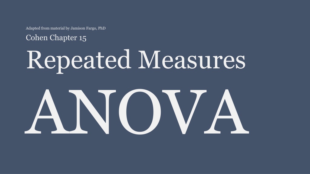
Adapted from material by Jamison Fargo, PhD
Cohen Chapter 15
ANOVA

“The biggest job we have is to teach a
newly hired employee how to
fail
intelligently. We have to train him to
experiment over and over and to keep
on trying and failing until he learns
what will work.”
Charles Kettering, American engineer, 1876 - 1958
One-Way
Repeated Measures ANOVA
4
Dr. Pearson is interested in determining whether the average man wants to
express his worries to his wife more (or less) the longer they are married.
The Desire to Express Worry (DEW) scale is administered to men when
they initially get married and then at their 5
th
, 10
th
, and 15
th
wedding
anniversaries.
What is the repeated-measures factor and what are its levels?
What is the outcome variable?
5
Design Types
1.
Same outcome, same cases,
different occasions
Time points
are levels of factor
2.
Different outcomes
(all on same metric) on
same cases
Different
outcomes
are levels of
factor
3.
Same outcome, different condition/exposure, on
cases that are
matched into sets
prior to
random assignment
Different
conditions
are levels of
factor
6
Experimental
Quasi-experimental
Field/Naturalistic studies
Longitudinal/Developmental studies
More powerful:
•
Each case serves as their
own control
, less
between-subject variation
•
Error term (denominator) of
F
-test for RM
ANOVA is often
less
than in Independent
Groups ANOVA
More economical:
•
Fewer cases
required
•
Independent Groups ANOVA:
•
3 conditions,
•
10 cases per condition
•
= 30 cases
•
RM ANOVA:
•
3 conditions,
•
same 10 cases used in all conditions
•
= 10 cases
7
Repeated-Measures (RM) factor
often referred to as:
‘Within-Subjects’ factor
Time 1, Time 2, Time 3, etc…
Condition1, Condition2, Condition3, etc…
May have…
Multiple RM factors
Factorial RM ANOVA
A combination of RM and independent groups
factors
Mixed Design ANOVA
Lack of independence of observations
must
be
accounted for in analysis
Time
as a RM Factor
Can answer questions such as:
Do measurements on outcome change over time or conditions?
Is change linear? Quadratic?
Is change positive or negative?
Does change 1
st
increase, then decrease (or vice versa)?
How long does change last?
Is change permanent over duration of study?
Is outcome same at beginning and end of study?
•
Researcher chooses
when
and
how frequently
to observe outcome,
time
is not
traditionally considered experimental variable
•
Not a manipulated factor, cannot counterbalance time, or randomize participants to have different times
or orders of observation
•
Although many experiments are longitudinal, they include an additional treatment variable that is
experimentally manipulated
•
Time intervals must be
equally spaced
•
If spacing is unequal, ANOVA with
random-effects must be used instead
8
Condition
as
the
RM Factor
9
Time
as a
RM Factor
Simultaneous RM Factors
•
Sometimes levels of RM factors are administered:
simultaneously
or
inter-mixed
within one experimental or observational study
For example…
•
Levels of RM factor might be verbs, nouns, and adjectives, which appear
randomly within a passage to be memorized
•
# of words of each type recalled by participants are recorded
10
Carryover Effects:
The Problem
…
•
Exposure to treatment or participation in
study/outcome at one time
influences
responses at
another
•
Biases related to practice, fatigue, etc.
•
When
time
is RM factor, carryover effects
are the
focus
of study
•
Learning, change over time
•
When
CONDITION
is RM factor and participants
rotate through conditions,
carryover effects are
not of
interest
and may lead to spurious results
•
Magnitude of carryover effects will vary across
treatment order
•
Differential carryover effects are very problematic
•
Effect of some levels of RM factor are more long-
lasting than others
11
•
Counterbalancing
: Varying RM condition order across
subjects
•
3-level RM factor: ABC, ACB, BCA, BAC, CAB, CBA
•
Partial counterbalancing
(Latin Squares): Too many possible
orders of RM conditions so a representative set is used
•
Each subject receives a
random order
of RM conditions
•
Each subject receives a
‘run-in’ period
(a series of practice
trials) at beginning of study to ‘stabilize’ performance
•
Intervening (
distractor
, neutral) trials between conditions
•
Larger time interval,
washout period
, between conditions
•
Note: Effects may not be eliminated by any of these methods
12
Carryover Effects:
Possible Solutions
Matched Designs
•
Alternative to having same cases engage in all RM conditions
•
Used to limit problems associated with…
•
Confounding variables (e.g., age, sex, education)
•
Other threats to internal validity associated with RM studies, such as carryover effects or ordering
•
Each member of a
set
of unique, but similar or matched, participants is
randomly assigned
to one
condition
•
In analysis, each
set of participants
treated
as if
they are the
same
participant
•
Participants matched into sets on
potentially confounding variables
(e.g., pretest scores, other
characteristics) prior to random assignment
•
Researcher may have too much faith in matching
•
Need to report on process used for matching
•
Usually only match (if at all) on 1 or 2 variables
13
May match and conduct 1-Way Independent Groups ANOVA to be more conservative in statistical results
•
Factor 1: RM or Within-Subjects factor: Time,
Condition
•
Factor 2: Subject factor: 8 participants = 8 levels
•
Only made with respect to marginal means of
RM
factor
•
Same form as 1-Way Independent Groups ANOVA
•
H
0
:
μ
1
=
μ
2
=…=
μ
k
•
H
1
:
H
0
is not true
14
Hypothesis:
1-Way RM ANOVA
is actually a
2-Way Independent Groups ANOVA
in disguise!!
Partitioning Variance
•
RM factor
: Same or similar outcome is measured more than once (each level)
by multiple participants
•
Subject factor
: Same or similar outcome is measured more than once (each
level) by same participants or sets of matched participants
•
RM x Subject factor
interaction
Total variation partitioned into 3 parts…but no SS
W
or error term!
SS
Total
=
SS
RM
+
SS
Subj
+
SS
RMxSubj
Note:
only 1 score per cell (n = 1) in previous 1-Way RM ANOVA
cross-classification, thus, no variability
within cells;
SS
W
= 0
•
SS
RMxSubj
is used as error term and represents variation in outcome
explained by…
1.
Interaction of participants with levels of RM factor
2.
Random (i.e., left-over) variation (error)
15
SS
Repeated Measure
In computing column or marginal means of RM factor all scores
in a given level are averaged regardless of row
•
n
k
= # participants per RM level
16
SS
Subject
•
In computing individual subject means, all scores in a given
row are averaged, regardless of level of RM factor
•
n
row
= # repeated measurements of outcome from same participant, since n = 1 per
cell
17
SS
interaction
18
•
Variability among cell means when variability due to
individual Subject and RM effects have been
removed
SS
Total
=
SS
Row
+
SS
Within
SS
Total
=
SS
RM
+
SS
Subj
+ SS
RMxS
19
SS & DEGREE OF FREEDOM
Independent Groups ANOVA
Repeated Measures ANOVA
MS
Subj
= SS
Subj
/ df
Subj
•
Generally
ignored
, considered nuisance variable
•
However, may be of interest to know if participants vary significantly on outcome:
•
Considered
‘random effect’
•
assumed participants (which serve as levels) are a random sample
•
Correct analysis is random- or mixed-effects ANOVA
•
Mixed-effects ANOVA
: Includes both fixed and random effects (which can either be
independent or repeated)
•
Mixed-design ANOVA
: Includes
both
independent (between-subjects) and repeated-
measures (within-subjects) factors
20
MS
RM*S
= SS
RM*S
/ df
RM*S
•
Not always of inferential interest
•
Useful for
testing assumptions
(later)
•
Indicates whether RM effect is
similar for all participants
•
When
MS
RMxS
= 0
, effect of RM factor is consistent across participants
desirable
•
When
MS
RMxS
is
large
, effect of RM factor likely differs across participants
undesirable
•
Line plot
of individual participant means across conditions/time can shed light
•
Variation due to participants (
MS
Subj
) is not included in error term for
F
-test of RM factor,
MS
RMxS
•
Thus, error term
is generally smaller in RM ANOVA than Independent Groups ANOVA
•
However, when matching leads to no variation across subjects (
SS
Subj
≈ 0) and
MS
RMxS
=
MS
Within
•
Results of RM ANOVA same as Independent Groups ANOVA
•
Increased effect of matching or repeating participants
•
SS
RMxS
decreases,
SS
Subj
increases
•
Decreased effect of matching or repeating participants
•
SS
RMxS
increases,
SS
Subj
decreases
21
SS
Within
=
SS
Subj
+
SS
RMxS
1-Way RM ANOVA: Summary Table
22
Assumptions
•
Participants are a
random
sample
from population and are
independent
of
one another (
Although participant observations are dependent, participants themselves are
independent)
•
DV
normally
distributed in the population
Less concerned: equal
n
per level and
df
Intrx
≈ 20 (CLT)
investigate via plotting
•
Homogeneity
of variance
Variance of DV is similar for all levels of RM factor
Leven’s or visual inspection
•
If
Time
is RM factor, data are measured at (near)
equal intervals
•
**Sphericity**
and
Compound symmetry
CS is a special case of sphericity
•
If CS is satisfied, sphericity is satisfied
•
However, if CS is
not
satisfied, sphericity may still be satisfied
23
Sphericity
•
Informally, it is the degree of violation of
independence same
for all levels of RM factor?
•
Taking DV, difference scores can be calculated for each participant between all possible pairs of
levels of RM factor
•
A variance can be calculated for each set of difference scores
•
When assumption of sphericity is met, difference score variances will be equal
•
Mauchly’s test of sphericity
•
Based on
χ
2
distribution
•
H
0
: Variances of difference scores between all pairs of levels of RM factor are equal
(sphericity)
•
Test not extremely useful as most “tests of other tests” tend to be…misleading*
•
Small N =
↑
Type II error
•
Large N, non-normality,
+
heterogeneity of covariances =
↑
Type I error
•
When using this test, assess all RM main effect(s)
•
Rule of thumb:
cause for concern may exist when the
largest variance is 4x greater than
smallest
24
*Kesselman, Rogan, Mendoza, & Breen, 1980
Sphericity: Mauchly’s test
Only applies to RM factors with > 2
levels
•
Cannot compare variances of difference
scores when there is only 1 set of
differences
•
Sphericity always met when
k
= 2 (RM
factor)
When violated,
↑
risk of Type I error
•
Critical
F
-statistics will be too small
•
F
-test is
+ biased
when sphericity is
violated
•
Several “alternatives”, discussed later
25
Compound Symmetry
A bit stricter than sphericity, which is a special case, and is subsumed by CS
Homogeneity of
variances
of difference scores
•
Variance of difference scores assumed to be equal
•
Same as previously mentioned for sphericity
Homogeneity of
covariances
of difference scores
•
Covariances of difference scores
(between all possible pairs of levels of the RM factor) assumed to be equal
•
Most software does
not assess this assumption
Additivity
(discussed in later slides)
26
27
Independence
Compound Symmetry
Groups or levels are
independent
of one
another as there are different participants
in each level; variances are non-0 and
assumed equal,
covariances are 0
Groups or levels are dependent or correlated.
Variances are non-0 and assumed
equal as
are covariances
(assumption met)
Additivity
•
Error term for RM ANOVA is
RMxS
interaction
•
Should only represent random error, not error plus variation of subjects over time or across conditions
•
Possible that effect of level A of RM factor is different for different subjects, and thus an interaction
between RM and S truly exists
•
Then, some of what we consider to be error when we calculate RMxS, is really an interaction effect, and
not just random error
•
Thus,
Additivity = absence of RMxS interaction
•
Presence of such an interaction indicates a multiplicative or nonadditive effect where different participants
have different patterns of response to RM factor
•
Error term is thus distorted by inclusion of a systematic (non-random) source of variation (due to
Subjects
)
•
Must determine what extraneous (between-subjects) factor (e.g., Gender) is causing interaction and test it
explicitly (e.g., Gender X RM Factor interaction)
•
Inclusion removes effects from error term (
MS
Intrx
)
->
Mixed-Design ANOVA
(
discussed next lecture
)
•
Since
nonadditivity
implies
heterogeneous variances for difference scores
, sphericity assumption will be
violated if this assumption is not met
•
A test exists for this assumption, called the “Tukey test for nonadditivity”, available in
additivityTests
::
tukey.test
()
Assessing Assumptions
If we want to assess these assumptions, we rely on results of the following approaches in practice:
•
Homogeneity of variances
•
Levene’s
(or Bartlett’s) test
•
car
::
leveneTest
()
•
Sphericity/Compound Symmetry
•
Mauchly test
•
Examination of variance-covariance matrix
•
Examination of variances among pairs of difference scores
•
Built intio
afex
::
aov_4
()
•
Additivity
•
Small
MS
Intrx
•
Individual Subject lines in a means
plot are mostly
parallel
•
additivityTests
::
tukey.test
()
29
Violations of Assumptions
Mostly concerned with
sphericity
-- > If violated, should pursue some alternative
30
If sphericity is met, 5 options:
•
Use
standard univariate
F-tests
(recommended)
•
Use
trend analysis
(recommended,
IF
this is
the goal)
•
Use a multivariate test (not recommended as
findings should be same as standard univariate
F-tests)
•
USE A
MAXIMUM LIKELIHOOD
PROCEDURE (HIGHLY RECOMMENDED)
•
Use a (not recommended, less power)
nonparametric test …
Friedman test (1-way
only)
If sphericity is NOT met, 5 options:
•
Use an
adjusted or alternative
F-test
(recommended)
•
Use
trend analysis
(recommended, if this is the
goal)
•
Use a multivariate test (less recommended in
most cases)
•
USE A
MAXIMUM LIKELIHOOD
PROCEDURE
(HIGHLY RECOMMENDED)
•
Use a
nonparametric test
(recommended, as a
last resort)…Friedman test (1-way only)
PSY 7650
MLM, HLM
Alternatives
Standard univariate
F
-tests are
not
recommended when sphericity is
violated
•
As mentioned before, will be too liberal and inaccurate (increased risk for Type I error)
Trend analysis
•
Sphericity assumption
irrelevant
•
Series of smaller
pairwise
comparisons across levels of the RM factor
•
Preferred for questions regarding the
shape
of the pattern in the DV over time
31
Adjusted or alternative univariate
F
-tests
(
Useful for
“smaller” N)
•
DEGREES OF FREEDOM
(
numerator and denominator
) are REDUCED by
multiplying by
EPSILON
•
Epsilon
= an adjustment factor describing the magnitude of the departure from sphericity
•
If sphericity assumption is perfectly met, epsilon = 1
•
Epsilon < 1 indicates departure from sphericity
•
Lower-bound depends on
k
levels of RM factor
•
1 / (
k
– 1), thus when
k
= 3, epsilon can be as small as .50
•
MORE conservative
F
-critical value
•
df
correction
approaches have been
criticized as too conservative
,
•
increasing risk of Type II error, as they assume maximal heterogeneity among cells
Several approaches (most-to-least conservative)
•
Lower-bound:
Uses the lower bound estimate of epsilon in the
df
correction
•
Greenhouse-Geisser:
Considered conservative and tends to underestimate epsilon when
epsilon is close to 1 (danger for over-correction)
•
Huynh-Feldt
: Considered less conservative when true value of epsilon is
≥ .75; but also
overestimates sphericity
32
Multivariate
F
-tests
•
DV is treated as a
set of variables
, ignores (does not assume) sphericity;
•
Assumes
general covariance structure
•
Cost:
Less powerful than RM ANOVA
and should be
avoided
UNLESS…
•
k
is low (< 5) and
N
is > (15 +
k
) (or
k
is high (5 to 8) and
N
is > (30 +
k
)) , epsilon is low (< .70), and
correlations among levels of RM factor
are high
•
Computed on differences among means
•
Most often used in context of
non-experimental research
•
Different forms exist:
•
Pillai’s trace,
+
Wilk’s
λ
, Hotelling’s trace, Roy’s largest root
•
+
Preferred and most commonly used
•
All yield same result for 1-Way RM ANOVA
•
Additional assumptions
for multivariate
F
-tests
•
Difference scores are multivariately normally distributed in population
•
Difference scores on outcome for each pair of levels are normally distributed
•
Difference scores on outcome for each pair of levels are normally distributed at every combination
of the values of other factors
•
Difference scores from any one participant are independent from those of any other participant
•
Use multivariate
η
2
for main effect or interaction when using multivariate F-tests
•
Multivariate
η
2
= 1 – Wilk’s Lambda (
Λ
)
33
Maximum likelihood procedures
•
Mixed-effects, multilevel, or hierarchical linear models
•
Wave of the (present and) future
•
Structure of
variance-covariance matrix
is modeled explicitly
•
not assumed to follow compound symmetry (can be tested empirically)
•
Autoregressive, exchangeable, or unstructured correlational structures are but a few examples
34
Effect of N on results of the Mauchly test of sphericity
Could have large N, reject H
0
, apply corrections, which are only minimal and unlikely to affect
outcome of results
Could have small N, fail to reject H
0
, not apply corrections and obtain spurious results
If epsilon is near 1, a correction is probably
not
necessary; however, if epsilon is near the lower
bound, a correction is likely necessary
Could run both RM ANOVA (with corrections for sphericity) and Multivariate analyses and
r
eport analysis that is statistically significant as that analysis has the greater power given
the circumstances
Effect Size:
η
2
35
•
Little evidence for a RM factor X Subject
interaction
(
additivity met
)
(Keppel & Wickens, 2004)
•
Evidence for a RM factor X Subject
interaction
(
non-additivity
) (Myers
& Well, 1991)
•
Conservative or ‘lower bound’ estimate
Effect Size:
ω
2
36
•
Little evidence for a RM factor X Subject interaction
•
Evidence for a RM factor X Subject
interaction
•
Conservative or ‘lower bound’ estimate
In both equations,
N
= # independent participants or sets of participants
FACTORIAL
REPEATED MEASURES
ANOVA
Dr. Evans wishes to evaluate various coping strategies for pain.
He obtains 8 volunteers to come to the lab on 2 consecutive days. On both days,
the volunteers plunge their hands into freezing cold water for 90 seconds.
They rate how painful the experience is on a scale from 1 to 50 (not painful) after
30 seconds, then 60 seconds, and then 90 seconds.
On one day they are given pain avoidance instructions and on the other day they
are given concentration on pain instructions.
In order to counterbalance the design, 4 students are given the avoidance and 4
students are given the concentration strategy the 1
st
day, then switched the 2
nd
day.
What are the RM factors? What are their levels?
What is the outcome variable?
Generally, ‘Order’ would be another factor (not RM) that would need to be included in the
ANOVA. For our purposes, we will say that this factor had no effect.
38
Dr. Chapman wishes to examine the effect of drugs A and B
as well as their interaction on blood flow. Each drug has
two possible formulations (levels). Each participant
received each of the 4 possible combinations of the 2 drugs
over several days (A1B1, A1B2, A2B1, A2B2). The half-life of
each drug was such that there were no carry-over effects.
What are the RM factors? What are their levels?
What is the outcome variable?
39
Factorial RM ANOVA
Same/matched
participant
Factorial RM ANOVA
2 or more RM factors (no independent factors)
Separate error term
for each RM main effect
and for interaction(s) among RM factors
Error terms = RM effect being tested (main effect or interaction) x Subjects interaction
•
1
st
RM main effect error term =
RM
1
x Subjects intrx
•
2
nd
RM main effect error term =
RM
2
x Subjects intrx
•
RM
1
x
RM
2
interaction error term =
RM
1
x
RM
2
x Subjects intrx
41
Factorial RM ANOVA: Summary Table
42
Effect Size:
η
2
43
•
Little evidence for a RM factor X Subject interaction (additivity
met) (Keppel & Wickens, 2004)
•
Compute depending on effect of interest
•
Evidence for interaction (non-additivity)
•
Conservative or ‘lower bound’ estimate
•
Compute depending on effect of interest
•
Present the range
Effect Size:
ω
2
•
Little evidence for a RM factor X Subject interaction
•
Compute depending on effect of interest
In both equations,
N
= #
independent participants or
sets of participants
Multiple Comparisons
Similar procedures as other ANOVA designs
Different error term
technically required
for each RM
comparison
•
Error represents differences among participants across levels of RM factor + random error
•
When a contrast omits one or more levels of the RM factor, how do we know whether omnibus
error term represented by RM x Subjects factors still applies to remaining levels? Hard to say…
However, use of
MS
Intrx
as error term in
omnibus
multiple comparisons
is usually justified
•
i.e., Follow-up 1-Way RM ANOVAs for simple main effects following interaction
•
Similar to follow-up 1-Way Independent Groups ANOVAs following significant Factorial
ANOVA
Simple or pairwise comparisons
avoid this problem by use of paired-samples
t
-tests or trend
analysis procedures (
recommended
)
45
Non-Significant Interaction(s)
46
Simple or complex
comparisons among
marginal means (levels)
if
F
-test significant
•
Only significant RM main effects
•
Reduces to two 1-Way RM ANOVAs
•
Marginal means are contrasted
•
Paired-samples
t
-tests;
α
PC
adjustment
•
Trend analysis or polynomial contrasts
No further tests if
F
-test of main-effect indicates difference
Significant Interaction(s)
•
Visualize
: Plot means
•
Tests of simple (main) effects
•
Contrast means from levels of one RM factor within levels of another RM factor using 1-way
RM ANOVA, paired-samples
t
-tests, or polynomial contrasts
•
Avoid interpretation of main effects
•
Alternative: Tests of interaction contrasts
•
Create difference scores between levels of one factor within each level of another factor and
compare with paired-samples
t
-tests
•
Order dictates valence of difference scores
•
Results will indicate whether mean differences across one condition vary across levels of other
condition
47
Significant Interaction(s)
•
Direction of ‘simple effect’
testing determined by
researcher
•
Simple effects generally
tested for each level of
stratifying factor
•
Simple comparisons
•
Paired-samples
t
-tests
•
1-way RM ANOVA followed
by simple or complex
comparisons (e.g., Paired-
samples
t
-tests)
48
Reporting Results
•
Summary
information: sample means and either
SD
s,
SE
s,
CI
s
•
Effect size
measures for main effects or interactions (even if
non-significant)
•
Results of
post hoc
comparisons
•
Mean differences and interactions can be
graphically
depicted
49
Problems
•
Extraneous factors (internal validity)
•
Passage of time in longitudinal studies
•
Do conditions, equipment, experimenters, participants change (interest, practice, skills) over the course
of the study in ways that may invalidate results?
•
Need methodological control
•
Generalizability (external validity)
•
Using fewer participants, so sample is less representative of population
•
Poor matching, small
n,
violated assumptions
may lead to deflated power in
RM ANOVA so that its power is same as Independent Groups ANOVA
•
If a participant is
missing data
on outcome from any level of any RM factor, all
data from that participant is removed from analysis
•
Decreased
N
less power
•
However, easier to impute missing data in RM ANOVA than in randomized- or independent-
groups designs
•
Other outcome scores are available from participants with missing values
•
Imputation results in several data sets on which the same analysis is conducted and results are compared
50
Supplemental
MS
RM*S
52
Can use to calculate the ICC
https://www.youtube.com/watch?v=ubNF9QNEQLA&t=0s&list=WL&index=1
Repeated Measures ANOVA is a statistical method used in research to analyze data collected from the same subjects under different conditions or at multiple time points. This method allows for comparing means across various treatments or time intervals within the same group, offering insights into within-subject variations. Factors, outcome variables, and differences between Repeated Measures ANOVA and Independent Groups ANOVA are explained.

Download Presentation

Please find below an Image/Link to download the presentation.
The content on the website is provided AS IS for your information and personal use only. It may not be sold, licensed, or shared on other websites without obtaining consent from the author.If you encounter any issues during the download, it is possible that the publisher has removed the file from their server.
You are allowed to download the files provided on this website for personal or commercial use, subject to the condition that they are used lawfully. All files are the property of their respective owners.
The content on the website is provided AS IS for your information and personal use only. It may not be sold, licensed, or shared on other websites without obtaining consent from the author.
E N D
Presentation Transcript
Adapted from material by Jamison Fargo, PhD Cohen Chapter 15 Repeated Measures ANOVA
The biggest job we have is to teach a newly hired employee how to fail intelligently. We have to train him to experiment over and over and to keep on trying and failing until he learns what will work. Charles Kettering, American engineer, 1876 - 1958
One-Way Repeated Measures ANOVA
Dr. Pearson is interested in determining whether the average man wants to express his worries to his wife more (or less) the longer they are married. The Desire to Express Worry (DEW) scale is administered to men when they initially get married and then at their 5th, 10th, and 15th wedding anniversaries. What is the repeated-measures factor and what are its levels? What is the outcome variable? Dr. Fairchild wishes to compare reaction time differences for the three subtests of the Stroop Test in patients with Parkinson s Disease: Color, Word, and Color Word. What is the repeated-measures factor and what are its levels? What is the outcome variable? 4
Design Types 1. Same outcome, same cases, different occasions Time points are levels of factor Experimental Quasi-experimental Field/Naturalistic studies Longitudinal/Developmental studies 2. Different outcomes (all on same metric) on same cases Different outcomes are levels of factor 3. Same outcome, different condition/exposure, on cases that are matched into sets prior to random assignment Different conditions are levels of factor 6
More powerful: Repeated-Measures (RM) factor often referred to as: Within-Subjects factor Each case serves as their own control, less between-subject variation Error term (denominator) of F-test for RM ANOVA is often less than in Independent Groups ANOVA Time 1, Time 2, Time 3, etc Condition1, Condition2, Condition3, etc May have Multiple RM factors Factorial RM ANOVA A combination of RM and independent groups factors Mixed Design ANOVA More economical: Fewer cases required Independent Groups ANOVA: 3 conditions, 10 cases per condition = 30 cases RM ANOVA: 3 conditions, same 10 cases used in all conditions = 10 cases Lack of independence of observations must be accounted for in analysis 7
Time as a RM Factor Can answer questions such as: Do measurements on outcome change over time or conditions? Is change linear? Quadratic? Is change positive or negative? Does change 1st increase, then decrease (or vice versa)? How long does change last? Is change permanent over duration of study? Is outcome same at beginning and end of study? Researcher chooses when and how frequently to observe outcome, time is not traditionally considered experimental variable Not a manipulated factor, cannot counterbalance time, or randomize participants to have different times or orders of observation Although many experiments are longitudinal, they include an additional treatment variable that is experimentally manipulated Time intervals must be equally spaced If spacing is unequal, ANOVA with random-effects must be used instead 8
Treatment A1 s1 s2 s3 s4 s5 . A2 s1 s2 s3 s4 s5 . A3 s1 s2 s3 s4 s5 . Row Means . . . . Column Means GM Month Month 1 1 1 3 5 2 2.40 Month 2 3 4 3 5 4 3.80 Month 3 6 8 6 7 5 6.40 Row Means 3.33 4.33 4.00 5.67 3.67 4.20 Time as a RM Factor s1 s2 s3 s4 s5 Column Means Treatment A1 s1 s2 s3 s4 s5 . A2 s1 s2 s3 s4 s5 . A3 s1 s2 s3 s4 s5 . Row Means . . . Condition as the RM Factor . Column Means GM Month 9 Month 1 1 1 3 5 2 2.40 Month 2 3 4 3 5 4 3.80 Month 3 6 8 6 7 5 6.40 Row Means 3.33 4.33 4.00 5.67 3.67 4.20 s1 s2 s3 s4 s5 Column Means
Simultaneous RM Factors Sometimes levels of RM factors are administered: simultaneously or inter-mixed within one experimental or observational study For example Levels of RM factor might be verbs, nouns, and adjectives, which appear randomly within a passage to be memorized # of words of each type recalled by participants are recorded 10
Carryover Effects: The Problem Exposure to treatment or participation in study/outcome at one time influences responses at another Biases related to practice, fatigue, etc. When time is RM factor, carryover effects are the focus of study Learning, change over time When CONDITION is RM factor and participants rotate through conditions, carryover effects are not of interest and may lead to spurious results Magnitude of carryover effects will vary across treatment order Differential carryover effects are very problematic Effect of some levels of RM factor are more long- lasting than others 11
Carryover Effects: Possible Solutions Counterbalancing: Varying RM condition order across subjects 3-level RM factor: ABC, ACB, BCA, BAC, CAB, CBA Partial counterbalancing (Latin Squares): Too many possible orders of RM conditions so a representative set is used Each subject receives a random order of RM conditions Each subject receives a run-in period (a series of practice trials) at beginning of study to stabilize performance Intervening (distractor, neutral) trials between conditions Larger time interval, washout period, between conditions Note: Effects may not be eliminated by any of these methods 12
Matched Designs Alternative to having same cases engage in all RM conditions Used to limit problems associated with Confounding variables (e.g., age, sex, education) Other threats to internal validity associated with RM studies, such as carryover effects or ordering Each member of a set of unique, but similar or matched, participants is randomly assigned to one condition In analysis, each set of participants treated as if they are the same participant Participants matched into sets on potentially confounding variables (e.g., pretest scores, other characteristics) prior to random assignment Researcher may have too much faith in matching Need to report on process used for matching Usually only match (if at all) on 1 or 2 variables 13 May match and conduct 1-Way Independent Groups ANOVA to be more conservative in statistical results
1-Way RM ANOVA is actually a 2-Way Independent Groups ANOVA in disguise!! Factor 1: RM or Within-Subjects factor: Time, Condition Factor 2: Subject factor: 8 participants = 8 levels Hypothesis: Only made with respect to marginal means of RM factor Same form as 1-Way Independent Groups ANOVA H0: 1 = 2= = k H1: H0 is not true 14
Partitioning Variance RM factor: Same or similar outcome is measured more than once (each level) by multiple participants Subject factor: Same or similar outcome is measured more than once (each level) by same participants or sets of matched participants RM x Subject factor interaction Total variation partitioned into 3 parts but no SSW or error term! SSTotal = SSRM + SSSubj + SSRMxSubj Note: only 1 score per cell (n = 1) in previous 1-Way RM ANOVA cross-classification, thus, no variability within cells; SSW = 0 SSRMxSubj is used as error term and represents variation in outcome explained by 1. Interaction of participants with levels of RM factor 2. Random (i.e., left-over) variation (error) 15
SSRepeated Measure In computing column or marginal means of RM factor all scores in a given level are averaged regardless of row nk = # participants per RM level = + + ... ( + 2 2 2 [( k n ) ( ) ) ] SS X X X X X X 1 2 RM RM GM RM GM RMk GM 2 2 2 2 n n n n + + + ... X X X X 1 2 RM RM RMk = = = = = 1 1 1 1 i i i i SS RM n N k 16
SSSubject In computing individual subject means, all scores in a given row are averaged, regardless of level of RM factor nrow = # repeated measurements of outcome from same participant, since n = 1 per cell = + + ... ( + 2 2 2 [( ) ( ) ) ] SS n X X X X X X 1 2 Subj row Subject GM Subj GM N GM 2 2 2 2 n n n n + + + ... X X X X 1 2 Subj Subj N = = = = = 1 1 1 1 i i i i SS Subj n N row 17
SSinteraction Variability among cell means when variability due to individual Subject and RM effects have been removed = + + + 2 2 [( ) ( ) ... SS X X X X 11 12 RMxS cell GM cell GM 2 ( ) ] X X SS SS cell rc GM RM Subj 2 2 n n = + + ... SS X X 11 12 RMxS cell cell = = 1 1 i i 2 n X 2 n = + 1 i X SS SS cell rc RM Subj N = 1 i 18
SS & DEGREE OF FREEDOM Independent Groups ANOVA Repeated Measures ANOVA SSTotal = SSRow + SSWithin SSTotal = SSRM + SSSubj + SSRMxS TOTAL df = nT 1 TOTAL df = nT 1 Bet-Sub df = n 1 With-Sub df = n( c 1 ) Bet-group df = k 1 With-group df = nT k RM SubxRM df = c 1 df =( n - 1)( c 1 ) MSEffect Term MSError Term F= 19
MS Subj = SS Subj / df Subj Generally ignored, considered nuisance variable However, may be of interest to know if participants vary significantly on outcome: Considered random effect assumed participants (which serve as levels) are a random sample Correct analysis is random- or mixed-effects ANOVA Mixed-effects ANOVA: Includes both fixed and random effects (which can either be independent or repeated) Mixed-design ANOVA: Includes both independent (between-subjects) and repeated- measures (within-subjects) factors 20
MSRM*S = SS RM*S / df RM*S SSWithin= SSSubj + SSRMxS Not always of inferential interest Useful for testing assumptions (later) Indicates whether RM effect is similar for all participants When MSRMxS= 0, effect of RM factor is consistent across participants desirable When MSRMxS is large, effect of RM factor likely differs across participants undesirable Line plot of individual participant means across conditions/time can shed light Variation due to participants (MSSubj) is not included in error term for F-test of RM factor, MSRMxS Thus, error termis generally smaller in RM ANOVA than Independent Groups ANOVA However, when matching leads to no variation across subjects (SSSubj 0) and MSRMxS= MSWithin Results of RM ANOVA same as Independent Groups ANOVA Increased effect of matching or repeating participants SSRMxSdecreases, SSSubj increases Decreased effect of matching or repeating participants SSRMxS increases, SSSubj decreases 21
1-Way RM ANOVA: Summary Table SS df MS F p Source RM Subj X X X X X X X Error(RM x Subj) Total X 22
Assumptions Participants are a random sample from population and are independent of one another (Although participant observations are dependent, participants themselves are independent) DV normally distributed in the population Less concerned: equal n per level and dfIntrx 20 (CLT) investigate via plotting Homogeneity of variance Variance of DV is similar for all levels of RM factor Leven s or visual inspection If Time is RM factor, data are measured at (near) equal intervals **Sphericity** and Compound symmetry CS is a special case of sphericity If CS is satisfied, sphericity is satisfied However, if CS is not satisfied, sphericity may still be satisfied 23
Sphericity Informally, it is the degree of violation of independence same for all levels of RM factor? Taking DV, difference scores can be calculated for each participant between all possible pairs of levels of RM factor A variance can be calculated for each set of difference scores When assumption of sphericity is met, difference score variances will be equal Mauchly s test of sphericity Based on 2 distribution H0: Variances of difference scores between all pairs of levels of RM factor are equal (sphericity) Test not extremely useful as most tests of other tests tend to be misleading* Small N = Type II error Large N, non-normality, +heterogeneity of covariances = Type I error When using this test, assess all RM main effect(s) Rule of thumb: cause for concern may exist when the largest variance is 4x greater than smallest *Kesselman, Rogan, Mendoza, & Breen, 1980 24
Sphericity: Mauchlys test Only applies to RM factors with > 2 levels Cannot compare variances of difference scores when there is only 1 set of differences Sphericity always met when k = 2 (RM factor) 300 250 value When violated, risk of Type I error Critical F-statistics will be too small F-test is + biased when sphericity is violated Several alternatives , discussed later 200 150 week08 week12 week16 week20 time 25
Compound Symmetry A bit stricter than sphericity, which is a special case, and is subsumed by CS Homogeneity of variances of difference scores Variance of difference scores assumed to be equal Same as previously mentioned for sphericity Homogeneity of covariances of difference scores Covariances of difference scores (between all possible pairs of levels of the RM factor) assumed to be equal Most software does not assess this assumption Additivity (discussed in later slides) 26
Independence Compound Symmetry A B 0 sB2 0 0 C 0 0 sC2 0 D 0 0 0 sD2 A B C D sAD sAB sAC sD2 A sA2 B C D A sA2 B sBA C sCA D sDA sAB sB2 sCB sDB sAC sBC sC2 sDC 0 0 0 Groups or levels are independent of one another as there are different participants in each level; variances are non-0 and assumed equal, covariances are 0 Groups or levels are dependent or correlated. Variances are non-0 and assumed equal as are covariances (assumption met) 27
Additivity Error term for RM ANOVA is RMxS interaction Should only represent random error, not error plus variation of subjects over time or across conditions Possible that effect of level A of RM factor is different for different subjects, and thus an interaction between RM and S truly exists Then, some of what we consider to be error when we calculate RMxS, is really an interaction effect, and not just random error Thus, Additivity = absence of RMxS interaction Presence of such an interaction indicates a multiplicative or nonadditive effect where different participants have different patterns of response to RM factor Error term is thus distorted by inclusion of a systematic (non-random) source of variation (due to Subjects) Must determine what extraneous (between-subjects) factor (e.g., Gender) is causing interaction and test it explicitly (e.g., Gender X RM Factor interaction) Inclusion removes effects from error term (MSIntrx) -> Mixed-Design ANOVA (discussed next lecture) Since nonadditivity implies heterogeneous variances for difference scores, sphericity assumption will be violated if this assumption is not met A test exists for this assumption, called the Tukey test for nonadditivity , available in additivityTests::tukey.test()
Assessing Assumptions If we want to assess these assumptions, we rely on results of the following approaches in practice: Homogeneity of variances Levene s(or Bartlett s) test car::leveneTest() Sphericity/Compound Symmetry Mauchly test Examination of variance-covariance matrix Examination of variances among pairs of difference scores Built intio afex::aov_4() Additivity Small MSIntrx Individual Subject lines in a means plot are mostly parallel additivityTests::tukey.test() 29
Violations of Assumptions Mostly concerned with sphericity -- > If violated, should pursue some alternative If sphericity is met, 5 options: If sphericity is NOT met, 5 options: Use standard univariate F-tests (recommended) Use an adjusted or alternative F-test (recommended) Use trend analysis (recommended, IF this is the goal) Use trend analysis (recommended, if this is the goal) Use a multivariate test (not recommended as findings should be same as standard univariate F-tests) Use a multivariate test (less recommended in most cases) USE A MAXIMUM LIKELIHOOD PROCEDURE (HIGHLY RECOMMENDED) USE A MAXIMUM LIKELIHOOD PROCEDURE (HIGHLY RECOMMENDED) PSY 7650 MLM, HLM Use a (not recommended, less power) nonparametric test Friedman test (1-way only) Use a nonparametric test (recommended, as a last resort) Friedman test (1-way only) 30
Alternatives Standard univariate F-tests are not recommended when sphericity is violated As mentioned before, will be too liberal and inaccurate (increased risk for Type I error) Trend analysis Sphericity assumption irrelevant Series of smaller pairwise comparisons across levels of the RM factor Preferred for questions regarding the shape of the pattern in the DV over time 31
Adjusted or alternative univariate F-tests (Useful for smaller N) DEGREES OF FREEDOM (numerator and denominator) are REDUCED by multiplying by EPSILON Epsilon = an adjustment factor describing the magnitude of the departure from sphericity If sphericity assumption is perfectly met, epsilon = 1 Epsilon < 1 indicates departure from sphericity Lower-bound depends on k levels of RM factor 1 / (k 1), thus when k = 3, epsilon can be as small as .50 MORE conservative F-critical value df correction approaches have been criticized as too conservative, increasing risk of Type II error, as they assume maximal heterogeneity among cells Several approaches (most-to-least conservative) Lower-bound: Uses the lower bound estimate of epsilon in the df correction Greenhouse-Geisser: Considered conservative and tends to underestimate epsilon when epsilon is close to 1 (danger for over-correction) Huynh-Feldt: Considered less conservative when true value of epsilon is .75; but also overestimates sphericity 32
Multivariate F-tests DV is treated as a set of variables, ignores (does not assume) sphericity; Assumes general covariance structure Cost: Less powerful than RM ANOVA and should be avoidedUNLESS k is low (< 5) and N is > (15 + k) (or k is high (5 to 8) and N is > (30 + k)) , epsilon is low (< .70), and correlations among levels of RM factor are high Computed on differences among means Most often used in context of non-experimental research Different forms exist: Pillai s trace, +Wilk s , Hotelling strace, Roy s largest root All yield same result for 1-Way RM ANOVA +Preferred and most commonly used Additional assumptions for multivariate F-tests Difference scores are multivariately normally distributed in population Difference scores on outcome for each pair of levels are normally distributed Difference scores on outcome for each pair of levels are normally distributed at every combination of the values of other factors Difference scores from any one participant are independent from those of any other participant Use multivariate 2 for main effect or interaction when using multivariate F-tests Multivariate 2 = 1 Wilk s Lambda ( ) 33
Maximum likelihood procedures Mixed-effects, multilevel, or hierarchical linear models Wave of the (present and) future Structure of variance-covariance matrix is modeled explicitly not assumed to follow compound symmetry (can be tested empirically) Autoregressive, exchangeable, or unstructured correlational structures are but a few examples Effect of N on results of the Mauchly test of sphericity Could have large N, reject H0, apply corrections, which are only minimal and unlikely to affect outcome of results Could have small N, fail to reject H0, not apply corrections and obtain spurious results If epsilon is near 1, a correction is probably not necessary; however, if epsilon is near the lower bound, a correction is likely necessary Could run both RM ANOVA (with corrections for sphericity) and Multivariate analyses and report analysis that is statistically significant as that analysis has the greater power given the circumstances 34
Effect Size: 2 Little evidence for a RM factor X Subject interaction (additivity met) (Keppel & Wickens, 2004) SS = 2 Partial RM SS + SS RM Intrx Evidence for a RM factor X Subject interaction (non-additivity) (Myers & Well, 1991) Conservative or lower bound estimate SS SS SS + SS SS = = 2 RM RM + SS RM Subj Intrx Total 35
Effect Size: 2 Little evidence for a RM factor X Subject interaction ( ) df MS MS MS k + = 2 Partial RM RM Intrx ( ) ( ) df MS N MS RM RM Intrx RM Intrx Evidence for a RM factor X Subject interaction Conservative or lower bound estimate ( ) df MS MS MS N MS = 2 RM RM k Intrx + + ( ) ( ) ( ) df MS N MS RM RM Intrx RM Intrx Subj In both equations, N = # independent participants or sets of participants 36
FACTORIAL REPEATED MEASURES ANOVA
Dr. Evans wishes to evaluate various coping strategies for pain. He obtains 8 volunteers to come to the lab on 2 consecutive days. On both days, the volunteers plunge their hands into freezing cold water for 90 seconds. They rate how painful the experience is on a scale from 1 to 50 (not painful) after 30 seconds, then 60 seconds, and then 90 seconds. On one day they are given pain avoidance instructions and on the other day they are given concentration on pain instructions. In order to counterbalance the design, 4 students are given the avoidance and 4 students are given the concentration strategy the 1st day, then switched the 2nd day. What are the RM factors? What are their levels? What is the outcome variable? Generally, Order would be another factor (not RM) that would need to be included in the ANOVA. For our purposes, we will say that this factor had no effect. 38
Dr. Chapman wishes to examine the effect of drugs A and B as well as their interaction on blood flow. Each drug has two possible formulations (levels). Each participant received each of the 4 possible combinations of the 2 drugs over several days (A1B1, A1B2, A2B1, A2B2). The half-life of each drug was such that there were no carry-over effects. What are the RM factors? What are their levels? What is the outcome variable? 39
Factorial RM ANOVA RM 1 A1 s1 s2 s3 s4 s5 . . s1 s2 s3 s4 s5 . . s1 s2 s3 s4 s5 . . M A1 A2 s1 s2 s3 s4 s5 . . s1 s2 s3 s4 s5 . . s1 s2 s3 s4 s5 . . M A2 A3 s1 s2 s3 s4 s5 . . s1 s2 s3 s4 s5 . . s1 s2 s3 s4 s5 . . M A3 Subj Means . . . . . Row Means B1 M B1 Same/matched participant Cell M Cell SD B2 . . . . . M B2 RM2 Cell M Cell SD B3 . . . . . M B3 Cell M Cell SD Column Means GM
Factorial RM ANOVA 2 or more RM factors (no independent factors) Separate error term for each RM main effect and for interaction(s) among RM factors Error terms = RM effect being tested (main effect or interaction) x Subjects interaction 1st RM main effect error term = RM1x Subjects intrx 2nd RM main effect error term = RM2x Subjects intrx RM1x RM2 interaction error term = RM1x RM2 x Subjects intrx 41
Factorial RM ANOVA: Summary Table SS df MS X F X p X Source Subj RM1 Error(RM1 x Subj) X X RM2 Error(RM2 x Subj) RM1 x RM2 Error(RM1 x RM2 x Subj) X X X X Total X X X 42
Effect Size: 2 Little evidence for a RM factor X Subject interaction (additivity met) (Keppel & Wickens, 2004) Compute depending on effect of interest SS SS SS = 2 Partial or or 1 SS 2 RM xRM + 1 2 RM SS + RM SS + SS SS SS 1 1 2 2 1 2 1 2 RM RM xS RM RM xS RM xRM RM xRM xS Evidence for interaction (non-additivity) Conservative or lower bound estimate Compute depending on effect of interest SS SS SS SS SS = 2 or or 1 2 RM xRM SS 1 2 RM RM Total Total Total Present the range 43
Effect Size: 2 Little evidence for a RM factor X Subject interaction Compute depending on effect of interest = 2 Main RM effect: Partial df df MS ( ) MS MS MS 1 1 1 2 N MS RM RM RM xRM xSubj k + ( ) ( ) 1 1 1 1 1 RM RM RM xSubj RM RM xSubj In both equations, N = # independent participants or sets of participants = 2 Interaction between RM factors: Partial df df MS ( ) MS MS MS ) + 1 2 1 2 1 2 RM xRM RM xRM RM xRM xSubj k ( ( ) N MS 1 2 1 2 1 2 1 2 1 2 RM xRM Where RM factors only, not including levels due to participants. Example: 2x3 RM ANOVA, = 6 RM xRM = Number of cells in RM ANOVA factorial design; RM xRM RM xR M xSubj RM xRM RM xRM xSubj k 1 2 k
Multiple Comparisons Similar procedures as other ANOVA designs Different error term technically required for each RM comparison Error represents differences among participants across levels of RM factor + random error When a contrast omits one or more levels of the RM factor, how do we know whether omnibus error term represented by RM x Subjects factors still applies to remaining levels? Hard to say However, use of MSIntrxas error term in omnibus multiple comparisons is usually justified i.e., Follow-up 1-Way RM ANOVAs for simple main effects following interaction Similar to follow-up 1-Way Independent Groups ANOVAs following significant Factorial ANOVA Simple or pairwise comparisons avoid this problem by use of paired-samples t-tests or trend analysis procedures (recommended) 45
Non-Significant Interaction(s) Only significant RM main effects Reduces to two 1-Way RM ANOVAs Marginal means are contrasted Paired-samples t-tests; PC adjustment Trend analysis or polynomial contrasts B B1 M11 M21 M31 B2 M12 M22 M32 MB2 Marginals MA1 MA2 MA3 A1 A2 A3 Simple or complex comparisons among marginal means (levels) if F-test significant A Marginals MB1 No further tests if F-test of main-effect indicates difference 46
Significant Interaction(s) Visualize: Plot means Tests of simple (main) effects Contrast means from levels of one RM factor within levels of another RM factor using 1-way RM ANOVA, paired-samples t-tests, or polynomial contrasts Avoid interpretation of main effects Alternative: Tests of interaction contrasts Create difference scores between levels of one factor within each level of another factor and compare with paired-samples t-tests Order dictates valence of difference scores Results will indicate whether mean differences across one condition vary across levels of other condition 47
Significant Interaction(s) B Direction of simple effect testing determined by researcher B1 M11 M21 M31 B2 M12 M22 M32 MB2 Marginals MA1 MA2 MA3 A1 A2 A3 A Marginals MB1 Simple effects generally tested for each level of stratifying factor Simple comparisons Paired-samples t-tests 1-way RM ANOVA followed by simple or complex comparisons (e.g., Paired- samples t-tests) B B1 M11 M21 M31 B2 M12 M22 M32 MB2 Marginals MA1 MA2 MA3 A1 A2 A3 A Marginals MB1 48
Reporting Results Summary information: sample means and either SDs, SEs, CIs Effect size measures for main effects or interactions (even if non-significant) Results of post hoc comparisons Mean differences and interactions can be graphically depicted 49
Problems Extraneous factors (internal validity) Passage of time in longitudinal studies Do conditions, equipment, experimenters, participants change (interest, practice, skills) over the course of the study in ways that may invalidate results? Need methodological control Generalizability (external validity) Using fewer participants, so sample is less representative of population Poor matching, small n, violated assumptions may lead to deflated power in RM ANOVA so that its power is same as Independent Groups ANOVA If a participant is missing data on outcome from any level of any RM factor, all data from that participant is removed from analysis Decreased N less power However, easier to impute missing data in RM ANOVA than in randomized- or independent- groups designs Other outcome scores are available from participants with missing values Imputation results in several data sets on which the same analysis is conducted and results are compared 50


")
")
")