Real-Time Signal Processing in DSP Systems

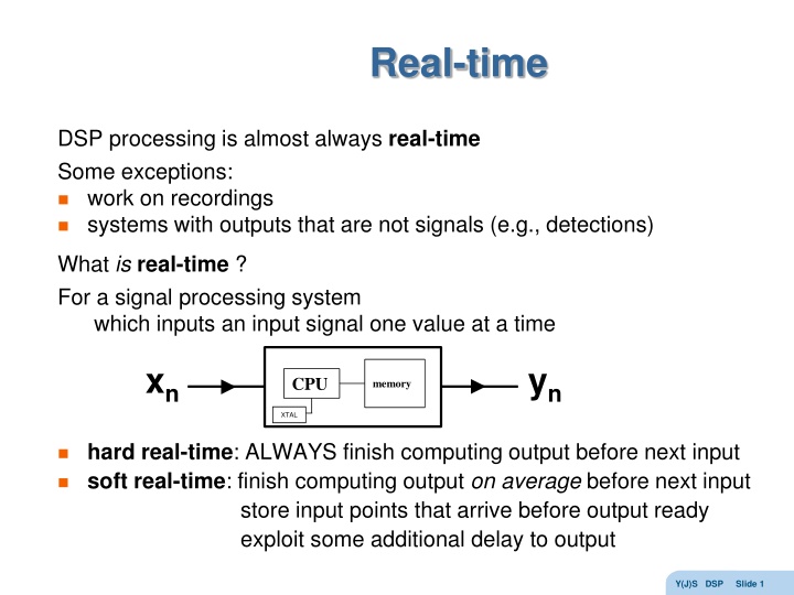
Real-time DSP processing is almost always real-time Some exceptions: work on recordings systems with outputs that are not signals (e.g., detections) What isreal-time ? For a signal processing system which inputs an input signal one value at a time xn yn CPU memory XTAL hard real-time: ALWAYS finish computing output before next input soft real-time: finish computing output on average before next input store input points that arrive before output ready exploit some additional delay to output Y(J)S DSP Slide 1

Example Assume samples arrive 1000 times per second fs = 1000 Hz then the time between samples is ts = 1 millisecond So, for hard real-time all of the processing of a single input sample xn in order to produce the output sample yn must take place in less than 1 millisecond (before the next sample xn+1 arrives) For soft real-time sometimes the processing of a single input sample xn can take longer than 1 millisecond in which case we store the next sample xn+1 until we output the output sample yn and then start processing xn+1 Y(J)S DSP Slide 2

DSP = Hard real-time In DSP we will only deal with hard real-time because we perform exactly the same computations each time (there are no conditionals) For example a x L = = l y MA filters n l n l 0 b y M AR filters (or ARMA) + = n n x y = m m n m 1 DFT ?? = ?=0 So, if we miss a deadline once it doesn t help to store the next input since the next input will also take too much time and the situation will only get worse and worse ? 1?? ?? ?? Y(J)S DSP Slide 3

Real-time for multi-input What about the DFT? We can t perform a DFT on one sample xn it only makes sense to perform on N samples x0, x1, x2, xN-1 ! For a system which performs calculation on N inputs hard real-time means that we must finish processing all N samples x0, x1, x2, xN-1 before the next N samples xN, xN+1, xN+2, x2N-1 arrive! The requirement is the same as before, but on average That is, finishing processing of N old samples during the time N new samples appear means on average processing a sample in a sampling time However, in general the processing of N samples need not reduce to N processing stages each on 1 sample! Y(J)S DSP Slide 4

Wrong way to process N samples You might think that we do the following: time 0: input x0, store in buffer, but don t perform any processing time 1: input x1, store in buffer, but don t perform any processing time N-1: input xN-1, store in buffer and perform all processing of N samples before the next sample xN arrives time N: input xN but don t perform any processing etc. but that would be really hard! We would need to process N samples in 1 sampling time although on average we need to process 1 sample per sample time So, what do we do instead? Y(J)S DSP Slide 5

Double buffering double buffer What we do is the following: time 0: input x0 into buffer 1 time 1: input x1 into buffer 1 time N-1: input xN-1 into buffer 1 (filling buffer) and start performing all processing of N samples in buffer 1 time N: input xN into buffer 2 and continue processing buffer 1 time N+1: input xN+1 into buffer 2 and continue processing buffer 1) some time before time 2N-1: finish processing buffer 1 and output time 2N-1: input x2N-1 into buffer 1 and start performing all processing of N samples in buffer 2 Trick: Instead of having to swap write pointers between buffer 1 and buffer 2 we can use a cyclic buffer 1 2 cyclic buffer 1 2 Y(J)S DSP Slide 6

Theorem for real-time The computational complexity of a real-time system that performs calculation on N inputs must not exceed O(N) In particular the DFT can not be performed in real-time since ?? = ?=0 requires computing N values X0, X1, , XN-1 each of which requires N multiplications (n = 0 N-1) and is thus O(N2) What does this theorem mean? Why can t we find a fast enough processor to perform anything we want in real-time? ? 1?? ?? ?? Y(J)S DSP Slide 7

The meaning of the theorem Imagine that you need to program some O(N2) process and as before samples arrive every millisecond Let s assume that you are told that N=1024 and that you manage to program you CPU to finish the processing in less than 1024 milliseconds But then it turns out that N=2048 is really needed You now have twice the time to perform the computation 2048 ms but because of O(N2) you require 4 times the time 4096 ms! So you buy a faster processor and manage to run in real-time but then if it turns out that N=4096 is needed no strong enough CPU is available! But if the complexity is O(N) then when N is increased from 1024 to 2048 you have twice the time to perform the computation but only need twice the time! Y(J)S DSP Slide 8

and the solution is DFT and iDFT are so critical in DSP that without a real-time implementation DSP won t work! The Fast Fourier Transform reduces the O(N2) complexity of the straightforward DFT to O(N log N) Note we don t need to specify the base of the log since changing base only inserts a multiplicative constant but we will always assume log2 But O(N log N) is higher than O(N) and so violates the theorem that real-time requires O(N) ! O(N log N) is not low enough to guarantee real-time for all N but is sufficiently low to enable even extremely large Ns DSP processors are rated by how large an FFT they can perform in real-time! Y(J)S DSP Slide 9

Warm-up problem #1 Find minimum and maximum of N numbers x0 x1 x2 x3 ...xN-2 xN-1 minimum alone takes N comparisons prove this maximum alone takes N comparisons prove this So we can certainly find both with 2N comparisons But there is a way to find both in 1 N comparisons x0 x1 x2 x3 ...xN-2 xN-1 smaller x0 x3 ...xN-1 larger x1 x2 ...xN-2 run over at pairs, separating into larger and smaller this takes N comparisons the minimum must be in the smaller list (why?) find it in N comparisons the maximum must be in the larger list find it in N comparisons altogether 3/2 N comparisons 25% savings for example Can we improve this by further decimation? Why not? Y(J)S DSP Slide 10

2 remarks this method uses decimation that is separating a sequence of N elements into two subsequences of N/2 elements based on even and odd elements although we reserved 2 buffers smaller x0 x3 ...xN-1 larger x1 x2 ...xN-2 the calculation can be performed in-place that is, without additional memory ! x0 x1 x2 x3 x4 x5 ...xN-2 xN-1 x0 x1 x3 x2 x5 x4 ...xN-2 xN-1 But to swap two values x0 x1 we do need an additional memory y x0 , x0 x1 ,x1 y why don t we count this? Y(J)S DSP Slide 11

Warm-up problem #2 Multiply two N digit numbers A and B (w.o.l.g. N binary digits) we saw that long multiplication is a convolution and thus takes 2N2 1-digit multiplications But there is a faster way! Partition the binary representation of A and B into 2 parts A7 A6 A5 A4 A3 A2 A1 A0 = AL AR B7 B6 B5 A4 B3 B2 B1 B0 = BL BR Now So partitioning factors reduces to 3/4 N2 saving 25% ! There s a small problem here the subtractions might add a bit! But O(3/4 N2) = O(N2) so we haven t changed the O complexity! Y(J)S DSP Slide 12

Continued But this time we can continue 0 0 1 3 multiplications, each N/2 bits 1 1 3 2 2 9 32 multiplications, each N/4 bits 27 log2(N) log2(N) 3 log2(N) multiplications, each 1 bit Now, 3log2(N) = Nlog So the complexity is O(Nlog2 2 3) O(N1.585) and O(N1.585) < O(N2) -- the O complexity has been reduced! log2 23 3 Why is alogk(b) = blog logk ka a ? This is the Karatsuba (special case of Toom-Cook) algorithm which was thought to be the fastest way to multiply until the FFT way was discovered Y(J)S DSP Slide 13

Toom-Cook example Let s multiply A=83 times B=122 using Toom Cook (the answer is 10,126) A = 0 1 0 1 0 0 1 1 B = 0 1 1 1 1 0 1 0 AL = 0 1 0 1 = 5 BL = 0 1 1 1 = 7 AR = 0 0 1 1 = 3 BR = 1 0 1 0 = 10 AR = = 5*7 *(256+16) + (5-3) * (10-7) *16 + 3*10*(16+1) = 35* 272 + Now for ALBL we repeat the process AL = 0 1 0 1 BL = 0 1 1 1 ALL = 0 1 = 1 BLL = 0 1 = 1 ALR = 0 1 = 1 BLR = 1 1 = 3 AL BL = 1*1*(16+4) + (1-1)*(3-1)*4 + 1*3*(4+1) and the same for the other 2 multiplications we then go one step further and have 9 individual bit multiplications 6 * 16 + 30* 17 Y(J)S DSP Slide 14

Decimation and Partition The two warm-up problems had a strategy in common If the complexity is C=cN2 then it is worthwhile to divide the input sequence into 2 subsequences Since performing the operation on each part costs c(N/2)2 = C/4 so the two together cost C/2 If we can glue the two parts back together in less than C/2 then we have a more efficient algorithm! But the two problems used two different methods of dividing the sequence x0 x1 x2 x3 x4 x5 x6 x7 Decimation x0 x2 x4 x6 x1 x3 x5 x7 LSB sort Partition x0 x1 x2 x3 x4 x5 x6 x7 MSB sort EVEN LEFT RIGHT ODD Y(J)S DSP Slide 15

Radix 2 In both warm-up problems, and in the FFT algorithm we will derive we divide up the sequence into 2 sub-sequences of length N/2 In fact we will require that N be a power of 2 so that we can continue to divide by 2 until we get to units Such algorithms are called radix-2 FFT algorithms We could also chose to divide it up into 3 subsequences or 4 or 5 or any other integer into which N factors There are special FFT algorithms for powers of other primes and for semi-primes like N=15=5*3 In fact, only for prime N is no possibility of reducing complexity Shmuel Winograd discovered FFTs with few multiplications for various values of N = N1 * N2 where N1 and N2 are coprime Y(J)S DSP Slide 16

Decimation in Time Partition in Frequency What does decimating a signal in the time domain do to the frequency domain representation ? Assume that the original signal x0 x1 x2 xN-1 was sampled at fs and thus by the sampling theorem have maximum frequency fN = fs/2 Then the decimated signals, x0 x2 x4 and x1 x3 x5 are sampled at fs/2 and thus have maximum frequency fs/4 So we obtain only the lower of the original spectral width in other words the LEFT partition of the spectrum Thus DIT = PIT We ll see later the exact relationship between the lower and upper partitions of the spectrum Y(J)S DSP Slide 17

Partition in Time Decimation in Frequency What does partitioning a signal in the time domain do to the frequency domain representation ? Assume that the original signal x0 x1 x2 xN-1 was sampled at fs and thus has duration T = N ts = N / fs Then the partitioned signals, x0 x1 xN/2-1 and xN/2 xN/2+2 xN-1 have duration N/2 ts = T/2 According to the uncertainty principle if the time duration t is reduced by then the frequency uncertainty is increased by 2 (the frequency resolution is blurred) So, we can effectively observe only every other spectral line! Thus PIT = DIT Y(J)S DSP Slide 18

FFT history The FFT has been discovered many times perhaps as early as unpublished 1805 work by Gauss which predates Fourier! In 1903 Runge discovered an FFT for N a power of 2 and in 1942 Danielson and Lanczos discovered a O(N log N) DFT However, credit is now usually given to John Wilder Tukey American mathematician/statistician (Princeton) who coined the words bit = binary digit and software James William Cooley American mathematician / programmer (IBM) who published in 1965 (in order to avoid patenting) The Cooley-Tukey algorithm is Decimation In Time that is, it decimates the signal in the time domain performing DFTs separately of the evens and the odds The Sande-Tukey algorithm is Decimation in Frequency that is, it partitions the signal in the time domain performing DFTs separately of the 1st half and 2nd half Y(J)S DSP Slide 19

Before starting Recall that the DFT is ?? = ?=0 where WN is the Nth root of unity WN = ? ?2 ? ? 1?? ?? ?? ? WN We will need three trigonometric identities 1. WNN = 1 (that s the definition!) WNN/2 = -1 (? ?2 ? WN2 =WN/2 (? ?2 ? WNN/2 ? 2= ? ? ?= -1 or ) 2. ? ?2=? ?2 ? 3. ?/2or ) WN WN2 =WN/2 They are trigonometric identities since WN = cos(2 ? ?) i sin(2 ? ?) Y(J)S DSP Slide 20

DIT (Cooley-Tukey) FFT Let s derive the radix-2 DIT FFT algorithm! We start by decimating the formula for the DFT that is, we separate the even terms 2n from the odd terms 2n+1 3rd identity 2n+1 k= WN nkand WN 2nk = WN/2 k WN 2nk and so we can rewrite: Now, WN DFT of evens DFT of odds Y(J)S DSP Slide 21

DIT the first step So we have found Odd Even which shows that the DFT indeed divides up into 2 half-sized DFTs and an additional N multiplications by WN This is encouraging, since the glue is O(N) ! k(for k=0 N-1) The glue factor is usually called the twiddle factor andit is the entire difference between the contribution of the two decimations to the original DFT k(k=0 N-1) Note that we precompute and store the N twiddle factors WN and don t have to compute them over and over again! Y(J)S DSP Slide 22

PIF The next step is to exploit the relationship between Decimation In Time and Partition In Frequency What is the connection between Xk in the left partition : 0 k N/2 1 and the corresponding component in the right partition Xk in the right partition : N/2 k N 1 2nd identity WNN/2 = -1 Note that we compute exactly the same products but add them with different signs + + + + + + + + Y(J)S DSP Slide 23

DIT is PIF So, we have already reduced the number of multiplications by Now, the products for which (-1)n is negative are odd n i.e., exactly those terms in the odd decimation! So We can draw this as a DSP diagram in a nice in-place way ! ? is the DFT sum ?? don t confuse it with ?? (it should have an intermediate sized x ) ? ! This reminds us of the N=2 butterfly but has a twiddle factor before the butterfly The DIF algorithm/s butterfly has a twiddle factor after the butterfly Y(J)S DSP Slide 24

DIT all the way We have already saved a factor of 2 in the multiplications but we needn't stop after splitting the original sequence in two ! Each half-length sub-sequence can be decimated again note that this is in-place! Assuming that N is a power of 2 we continue decimating until we get to the basic N=2 butterfly Note that since WN/2 = WN2 we can draw this k and we only have to keep one table of WN Y(J)S DSP Slide 25

Lets continue! Instead of explicitly writing equations for the next step it is easier to do everything graphically In order to make things simple, we ll assume N=8 and explicitly draw out all the steps decimate the N=8 sequence into two subsequences of length 4 decimate each of the sub-sequences of length 4 into two sub-sub-sequences of length 2 (4 altogether) perform four basic N=2 butterflies Let s see this happen! Y(J)S DSP Slide 26

DIT N=8 - step 0 Y(J)S DSP Slide 27

DIT N=8 - step 1 in-place! Y(J)S DSP Slide 28

DIT N=8 - step 1 : 4 butterflies The butterflies are all entangled do you see them? Y(J)S DSP Slide 29

DIT N=8 - step 2 W40 = W80 W41 = W82 Y(J)S DSP Slide 30

DIT N=8 - step 2 Note that the second stage butterflies are less entangled! Y(J)S DSP Slide 31

DIT N=8 - step 3 Y(J)S DSP Slide 32

Complexity An FFT of length N has log2(N) stages of butterflies there are N butterflies in each stage, each with 1 complex multiply 2 complex adds (1 add and 1 subtract) So there are : N log2(N) complex multiplications N log2(N) complex additions Which is why we say that the complexity is O(N log N) for N=8 there are 3 stages Stage 1: 4 butterflies Stage 2: 2*2 butterflies Stage 3: 4*1 butterflies stage 3 stage 2 stage 1 Y(J)S DSP Slide 33

Well, its even a bit less Actually, some of the multiplications are trivial! the first stage has one trivial multiplication (WN the 2nd stage has 2 trivial multiplications the last stage has no true multiplications (it has N=2 butterflies!) So for N=8 there are really only 5 multiplications instead of 8log2(8) = 24 ! 0=1) Y(J)S DSP Slide 34

Real complexity So far we have counted complex multiplications and additions Each complex add entails 2 real adds Each complex multiply is either: 4 real multiplies and 2 real adds (a + i b) (c + i d) = (a*c b*d) + i (a*d + b*c) or 3 real multiplies and 5 real adds M1 = a*c M2 = b*d M3 = (a+b)*(c+d) (a + i b) (c + i d) = (M1 M2) + i (M3 M2 M1) So N log2(N) complex additions = 2N log2(N) real additions N log2(N) complex multiplications = 2N log2(N) real multiplications and another N log2(N) real additions or 3/2 N log2(N) real multiplications and another 5/2 N log2(N) real additions Y(J)S DSP Slide 35

Whats going on? The order of the input values is very strange! Our time domain signal is not arranged x0, x1, x2, ! Y(J)S DSP Slide 36

Bit reversal Let s see if we can figure it out! Here for N=16 IN-PLACE! 1st transition is cyclic left shift 2nd transition freezes the LSB and cyclic left shifts the rest 3rd transition freezes the 2 LSBs and cyclic left shifts (swaps) the rest Altogether we find abcd bcda cdba The bits of the index have been reversed ! This is called bit-reversal and DSP processors have a special addressing mode for it dcba Y(J)S DSP Slide 37

DIT N=8 with bit reversal Y(J)S DSP Slide 38

The matrix interpretation The FFT can be understood as a matrix decomposition that reduces the number of operations to multiply by it For example, when N=4 The right matrix is a permutation matrix which carries out the bit reversal The middle matrix comprises the butterflies (note the block matrix form) The left matrix is the twiddle factors Y(J)S DSP Slide 39

What about the DIF algorithm? The other radix-2 FFT algorithm could be called Partition in Time but is always called Decimation In Frequency To derive it algebraically we need to return to the DFT formula and partition the sum into high and low halves We then exploit that DIF to relate Xk (even k) with Xk+1 resulting in butterflies But instead of working hard we ll use a trick! Performing the transposition theorem on the N=8 DIT(and a mirror reflection) gives us the n=8 DIF! Y(J)S DSP Slide 40

DIF N=8 DIF butterfly Y(J)S DSP Slide 41

FIFO FFT There are many other Fast Fourier Transform algorithms! What if we need to update the DFT every sample? In other words, [x0, x1, x2, xN-1], [x1, x2, x3, xN], [x2, x3, x4, xN+1], You might already know the trick on how to update a simple moving average A1 = x0 + x1 + x2+ + xN-1 A2 = x1 + x2 + x3+ + xN = A1 x0 + xN A3 = x2 + x3 + x4+ + xN+1 = A2 x1 + xN+1 This is implemented by maintaining a FIFO of length N adding the new input and subtracting the one to be discarded A similar trick works for weighted MA if the weights form a geometric progression A1 = x0 + q x1 + q2 x2+ + qN-1 xN-1 A2 = x1 + q x2 + q2 x3+ + qN-1 xN A3 = x2 + q x3 + q2 x4+ + qN-1 xN+1 = (A2 x1)/q + qN-1 xN+1 = (A1 x0)/q + qN-1 xN Y(J)S DSP Slide 42

FIFO FFT (cont) k The DFT is just such a weighted moving average, with q = WN but when moving from time to time we shouldn t reset the clock! So and hence requiring only 2 complex additions and one multiplication per k or altogether N multiplications and 2N additions! Y(J)S DSP Slide 43

Goertzels algorithm Sometimes we are only interested in the energy |Xk|2 of a few of the frequencies k and computing all N spectral values would be wasteful For example, when looking for energy at a few discrete frequencies as in a DTMF detector For such cases there is an algorithm due to Goertzel (Herzl in Russian) which is less expensive that running many bandpass filters The idea is to compute only the Xk needed by using Horner s rule for evaluating polynomials (simplify WN k to W) This can be further simplified to get a noncomplex recursion Y(J)S DSP Slide 44

Goertzel 1 To make the recursion look like a convolution we use V = W-1 Changing the overall phase doesn t change the power spectrum which using Horner s rule is coded like this : Since all the xn are real, at each step Pn Pn-1V is real So we implicitly define a new real sequence Qn by Pn = Qn - Qn-1W Y(J)S DSP Slide 45

Goertzel 2 After a little algebra we find the following recursion: And the desired energy is given by where Y(J)S DSP Slide 46

Using Goertzel To use Goertzel first decide on how many points N you want to use Since Goertzel s algorithm only works for integer digital frequencies (that is, for analog frequencies f = k/N fs) larger N allows finer resolution and narrower bandwidth but also longer computation time and delay For each frequency that is needed compute W and A initialize iterate N-1 times using A compute X using W compute the desired squared power using A Y(J)S DSP Slide 47

Other radixes While radix-2 is popular, sometimes other radixes are better The radix 4 DFT is which corresponds to radix-4 butterflies 12 complex additions 0 true multiplications which is more expensive than radix-2 8 complex additions 0 true multiplications Y(J)S DSP Slide 48

FFT842 But this is only the case for N=4 itself For powers of 4 there are only log4N= 1/2 log2N stages of butterflies and each has N complex multiplications and so only 3/8 log2Nmultiplicationsaltogether which is slightly less than log2N! But only half of the powers of 2 are also powers of 4 so the algorithm is less applicable Similarly, for N=8m there are even fewer stages but only a quarter of the powers of 2 are powers of 8 So, the FFT842 algorithm performs as many radix-8 stages that it can it then performs either a radix-4 or a radix-2 stage as needed It beats out pure radix-2 algorithms on general purpose CPUs but highly optimized radix-2 are preferable on DSPs Y(J)S DSP Slide 49

Multiplication by FFT When learning the Toom-Cook algorithm we said that for large N the FFT will multiply even faster That is because O(N log N) < O(Nlog2 23) We saw that long multiplication c = a*b is actually 2N convolutions Hence convolution in the time domain takes O(N2) multiplications but in the frequency domain it only takes O(N) So the strategy is instead of convolution c = a * b use the FFT to convert from the time to the frequency domain a A and b B [ O(N log N) ] multiply point by point in the frequency domain C=AB [ O(N) ] convert back from the frequency to the frequency domain C c [ O(N log N) ] Altogether O(N log N) ! Y(J)S DSP Slide 50