RAID Technology in DBMS: Redundancy and Performance
This content provides insights into RAID technology, discussing the combination of reliability and performance in managing multiple disks through various RAID levels like RAID 0, RAID 1, RAID 2, RAID 3, RAID 4, and RAID 5. It explores the advantages of RAID, such as data striping, mirroring, bit interleaving, and parity, highlighting the differences between RAID 4 and RAID 5 based on different write scenarios and disk expansion needs.

Download Presentation

Please find below an Image/Link to download the presentation.
The content on the website is provided AS IS for your information and personal use only. It may not be sold, licensed, or shared on other websites without obtaining consent from the author.If you encounter any issues during the download, it is possible that the publisher has removed the file from their server.
You are allowed to download the files provided on this website for personal or commercial use, subject to the condition that they are used lawfully. All files are the property of their respective owners.
The content on the website is provided AS IS for your information and personal use only. It may not be sold, licensed, or shared on other websites without obtaining consent from the author.
E N D
Presentation Transcript
Database Applications (15-415) DBMS Internals: Part II Lecture 13, February 25, 2018 Mohammad Hammoud
Today Last Session: DBMS Internals- Part I Today s Session: DBMS Internals- Part II A Brief Summary on Disks and the RAID Technology Disk and memory management Announcements: Project 2 is due on March 22 by midnight The Midterm exam is on March 13
DBMS Layers Queries Query Optimization and Execution Relational Operators Files and Access Methods Transaction Manager Recovery Manager Buffer Management Lock Manager Disk Space Management DB
Multiple Disks Discussions on: Reliability Performance Reliability + Performance
Redundant Arrays of Independent Disks A system depending on N disks is much more likely to fail than one depending on one disk If the probability of one disk to fail is f Then, the probability of N disks to fail is (1-(1-f)N) How would we combine reliability with performance? Redundant Arrays of Inexpensive Disks (RAID) combines mirroring and striping Nowadays, Independent!
RAID Level 0 Data Striping
RAID Level 1 Data Mirroring
RAID Level 2 Data Data bits Bit Interleaving; ECC Check bits
RAID Level 3 Data Data bits Bit Interleaving; Parity Parity bits
RAID Level 4 Data Data blocks Block Interleaving; Parity Parity blocks
RAID Level 5 Data Data and parity blocks Block Interleaving; Parity
RAID 4 vs. RAID 5 What if we have a lot of small writes? RAID 5 is better What if we have mostly large writes? Multiples of stripes Either is fine What if we want to expand the number of disks? RAID 5: add a disk, re-compute parity, and shuffle data blocks among all disks to reestablish the check-block pattern (expensive!)
Beyond Disks: Flash Flash memory is a relatively new technology providing the functionality needed to hold file systems and DBMSs It is writable It is readable Writing is slower than reading It is non-volatile Faster than disks, but slower than DRAMs Unlike disks, it allows random accesses Limited lifetime More expensive than disks
Disks: A Very Brief Summary DBMSs store data in disks Disks provide large, cheap, and non-volatile storage I/O time dominates! The cost depends on the locations of pages on disk (among others) It is important to arrange data sequentially to minimize seek and rotational delays
Disks: A Very Brief Summary Disks can cause reliability and performance problems To mitigate such problems we can adopt multiple disks and accordingly gain: 1. More capacity 2. Redundancy 3. Concurrency To achieve only redundancy we can apply mirroring To achieve only concurrency we can apply striping To achieve redundancy and concurrency we can apply RAID (e.g., levels 2, 3, 4 or 5)
DBMS Layers Queries Query Optimization and Execution Relational Operators Files and Access Methods Transaction Manager Recovery Manager Buffer Management Lock Manager Disk Space Management DB
Disk Space Management DBMSs disk space managers Support the concept of a page as a unit of data Page size is usually chosen to be equal to the block size so that reading or writing a page can be done in 1 disk I/O Allocate/de-allocate pages as a contiguous sequence of blocks on disks Abstracts hardware (and possibly OS) details from higher DBMS levels
What to Keep Track of? The DBMS disk space manager keeps track of: Which pages are on which disk blocks Which disk blocks are in use (i.e., occupied by data blocks) Blocks can be initially allocated contiguously, but allocating and de-allocating blocks usually create holes Hence, a mechanism to keep track of free blocks is needed A list of free blocks can be maintained (storage could be an issue) Alternatively, a bitmap with one bit per each disk block can be maintained (more storage efficient and faster in identifying contiguous free areas!)
OS File Systems vs. DBMS Disk Space Managers Operating Systems already employ disk space managers using their file abstraction Read byte i of file f read block m of track t of cylinder c of disk d DBMSs disk space managers usually pursue their own disk management without relying on OS file systems Enables portability Can address larger amounts of data Allows spanning and mirroring
DBMS Layers Queries Query Optimization and Execution Relational Operators Files and Access Methods Transaction Manager Recovery Manager Buffer Management Lock Manager Disk Space Management DB
Buffer Management What is a DBMS buffer manager? It is a software component responsible for managing (e.g., placing and replacing) data on memory (or buffer pool) It hides the fact that not all data is in the buffer pool Page Requests from Higher Levels Memory page = disk block Buffer pool in the main memory free frame choice of frame dictated by a replacement policy DB DISK
Satisfying Page Requests For each frame in the buffer pool, the DBMS buffer manager maintains: A pin_count variable: # of users of a page A dirty variable: whether a page has been modified or not If a page is requested and missed in the pool, the DBMS buffer manager: Chooses a frame for placement and increments its pin_count (a process known as pinning) If the frame is empty, fetches the page (or block) from disk and places it in the frame If the frame is occupied: If the hosted page is dirty, writes it back to the disk, then fetches and places the requested page in the frame Else, fetches and places the requested page in the frame
Replacement Policies A frame is not used to store a new page until its pin_count becomes 0 I.e., Until all requestors of the old page have unpinned it (a process known as unpinning) When many frames with pin_count = 0 are available, a specific replacement policy is pursued If no frame in the pool has pin_count = 0 and a page which is not in the pool is requested, the buffer manager must wait until some page is released!
Replacement Policies When a new page is to be placed in the pool, a resident page should be evicted first Criterion for an optimum replacement [Belady, 1966]: The page that will be accessed farthest in the future should be the one that is evicted Unfortunately, optimum replacement is not implementable! Hence, most buffer managers capitalize on a different criterion E.g., The page that was accessed the farthest back in the past is the one that is evicted, leading to a policy known as Least Recently Used (LRU) Other policies: MRU, Clock, FIFO, and Random, among others
Example: LRU LRU Chain: 7 0 1 2 0 3 0 4 2 3 0 3 2 1 2 0 1 7 0 1 Reference Trace Pool X (size = 3) Pool Y (size = 4) Pool Z (size = 5) Frame 0 Frame 1 Frame 2 Frame 3 Frame 4 # of Hits: # of Misses: # of Hits: # of Misses: # of Hits: # of Misses:
Example: LRU LRU Chain: 7 7 0 1 2 0 3 0 4 2 3 0 3 2 1 2 0 1 7 0 1 Reference Trace Pool X (size = 3) Pool Y (size = 4) Pool Z (size = 5) Frame 0 7 7 7 Frame 1 Frame 2 Frame 3 Frame 4 # of Hits: # of Misses: 1 # of Hits: # of Misses: 1 # of Hits: # of Misses: 1
Example: LRU LRU Chain: 0 7 7 0 1 2 0 3 0 4 2 3 0 3 2 1 2 0 1 7 0 1 Reference Trace Pool X (size = 3) Pool Y (size = 4) Pool Z (size = 5) Frame 0 7 7 7 Frame 1 0 0 0 Frame 2 Frame 3 Frame 4 # of Hits: # of Misses: 2 # of Hits: # of Misses: 2 # of Hits: # of Misses: 2
Example: LRU LRU Chain: 1 0 7 7 0 1 2 0 3 0 4 2 3 0 3 2 1 2 0 1 7 0 1 Reference Trace Pool X (size = 3) Pool Y (size = 4) Pool Z (size = 5) Frame 0 7 7 7 Frame 1 0 0 0 1 1 1 Frame 2 Frame 3 Frame 4 # of Hits: # of Misses: 3 # of Hits: # of Misses: 3 # of Hits: # of Misses: 3
Example: LRU LRU Chain: 2 1 0 7 7 0 1 2 0 3 0 4 2 3 0 3 2 1 2 0 1 7 0 1 Reference Trace Pool X (size = 3) Pool Y (size = 4) Pool Z (size = 5) Frame 0 7 7 2 Frame 1 0 0 0 1 1 1 Frame 2 2 2 Frame 3 Frame 4 # of Hits: # of Misses: 4 # of Hits: # of Misses: 4 # of Hits: # of Misses: 4
Example: LRU LRU Chain: 0 2 1 7 7 0 1 2 0 3 0 4 2 3 0 3 2 1 2 0 1 7 0 1 Reference Trace Pool X (size = 3) Pool Y (size = 4) Pool Z (size = 5) Frame 0 7 7 2 Frame 1 0 0 0 1 1 1 Frame 2 2 2 Frame 3 Frame 4 # of Hits: 1 # of Misses: 4 # of Hits: 1 # of Misses: 4 # of Hits: 1 # of Misses: 4
Example: LRU LRU Chain: 3 0 2 1 7 7 0 1 2 0 3 0 4 2 3 0 3 2 1 2 0 1 7 0 1 Reference Trace Pool X (size = 3) Pool Y (size = 4) Pool Z (size = 5) Frame 0 7 3 2 Frame 1 0 0 0 1 1 3 Frame 2 2 2 Frame 3 3 Frame 4 # of Hits: 1 # of Misses: 5 # of Hits: 1 # of Misses: 5 # of Hits: 1 # of Misses: 5
Example: LRU LRU Chain: 0 3 2 1 7 7 0 1 2 0 3 0 4 2 3 0 3 2 1 2 0 1 7 0 1 Reference Trace Pool X (size = 3) Pool Y (size = 4) Pool Z (size = 5) Frame 0 7 3 2 Frame 1 0 0 0 1 1 3 Frame 2 2 2 Frame 3 3 Frame 4 # of Hits: 2 # of Misses: 5 # of Hits: 2 # of Misses: 5 # of Hits: 2 # of Misses: 5
Example: LRU LRU Chain: 4 0 3 2 1 7 7 0 1 2 0 3 0 4 2 3 0 3 2 1 2 0 1 7 0 1 Reference Trace Pool X (size = 3) Pool Y (size = 4) Pool Z (size = 5) Frame 0 4 3 4 Frame 1 0 0 0 1 4 3 Frame 2 2 2 Frame 3 3 Frame 4 # of Hits: 2 # of Misses: 6 # of Hits: 2 # of Misses: 6 # of Hits: 2 # of Misses: 6
Example: LRU LRU Chain: 2 4 0 3 1 7 7 0 1 2 0 3 0 4 2 3 0 3 2 1 2 0 1 7 0 1 Reference Trace Pool X (size = 3) Pool Y (size = 4) Pool Z (size = 5) Frame 0 4 3 4 Frame 1 0 0 0 1 4 2 Frame 2 2 2 Frame 3 3 Frame 4 # of Hits: 2 # of Misses: 7 # of Hits: 3 # of Misses: 6 # of Hits: 3 # of Misses: 6
Example: LRU LRU Chain: 3 2 4 0 1 7 7 0 1 2 0 3 0 4 2 3 0 3 2 1 2 0 1 7 0 1 Reference Trace Pool X (size = 3) Pool Y (size = 4) Pool Z (size = 5) Frame 0 4 3 4 Frame 1 0 0 3 1 4 2 Frame 2 2 2 Frame 3 3 Frame 4 # of Hits: 2 # of Misses: 8 # of Hits: 4 # of Misses: 6 # of Hits: 4 # of Misses: 6
Example: LRU LRU Chain: 0 3 2 4 1 7 7 0 1 2 0 3 0 4 2 3 0 3 2 1 2 0 1 7 0 1 Reference Trace Pool X (size = 3) Pool Y (size = 4) Pool Z (size = 5) Frame 0 4 3 0 Frame 1 0 0 3 1 4 2 Frame 2 2 2 Frame 3 3 Frame 4 # of Hits: 2 # of Misses: 9 # of Hits: 5 # of Misses: 6 # of Hits: 5 # of Misses: 6
Observation: The Stack Property Adding pool space never hurts, but it may or may not help This is referred to as the Stack Property LRU has the stack property, but not all replacement policies have it E.g., FIFO does not have it
Working Sets Given a time interval T, WorkingSet(T) is defined as the set of distinct pages accessed during T Its size (or what is referred to as the working set size) is all what matters It captures the adequacy of the cache size with respect to the program behavior What happens if a process performs repetitive accesses to some data in memory, with a working set size that is larger than the buffer pool?
The LRU Policy: Sequential Flooding To answer this question, assume: Three pages, A, B, and C An access pattern: A, B, C, A, B, C, etc. A buffer pool that consists of only two frames Access C: Access A: Access B: Access A: Access B: Access C: Access A: . . . B A C B A A C C B B A A C Page Fault Page Fault Page Fault Page Fault Page Fault Page Fault Page Fault Although the access pattern exhibits temporal locality, no locality was exploited! This phenomenon is known as sequential flooding For this access pattern, MRU works better!
Why Not Virtual Memory of OSs? Operating Systems already employ a buffer management technique known as virtual memory Virtual Address Virtual Pages Page # Offset 68K-76k --- 60K-68k --- 52K-60k --- 44K-52k Physical Pages Virtual Address Space --- 32K-40k 16K-24k 16K-24k 8K-16k --- 8K-16k 0K-8k 0K-8k Physical Address Space
Why Not Virtual Memory of OSs? Nonetheless, DBMSs pursue their own buffer management so that they can: Predict page reference patterns more accurately and applying effective strategies (e.g., page prefetching for improving performance) Force pages to disks Needed for the WAL protocol Typically, the OS cannot guarantee this!
DBMS Layers Queries Query Optimization and Execution Relational Operators Files and Access Methods Transaction Manager Recovery Manager Buffer Management Lock Manager Disk Space Management DB
Records, Pages and Files Higher-levels of DBMSs deal with records (not pages!) At lower-levels, records are stored in pages But, a page might not fit all records of a database Hence, multiple pages might be needed A File A collection of pages is denoted as a file A Record A Page
File Operations and Organizations A file is a collection of pages, each containing a collection of records Files must support operations like: Insert/Delete/Modify records Read a particular record (specified using a record id) Scan all records (possibly with some conditions on the records to be retrieved) There are several organizations of files: Heap Sorted Indexed
Heap Files Records in heap file pages do not follow any particular order As a heap file grows and shrinks, disk pages are allocated and de-allocated To support record level operations, we must: Keep track of the pages in a file Keep track of the records on each page Keep track of the fields on each record
Supporting Record Level Operations Keeping Track of Pages in a File Fields in a Record Records in a Page
Heap Files Using Lists of Pages A heap file can be organized as a doubly linked list of pages Data Page Data Page Data Page Full Pages Header Page Available Page Available Page Available Page Pages with Free Space The Header Page (i.e., <heap_file_name, page_1_addr> is stored in a known location on disk Each page contains 2 pointers plus data
Heap Files Using Lists of Pages It is likely that every page has at least a few free bytes Thus, virtually all pages in a file will be on the free list! To insert a typical record, we must retrieve and examine several pages on the free list before one with enough free space is found This problem can be addressed using an alternative design known as the directory-based heap file organization
Heap Files Using Directory of Pages A directory of pages can be maintained whereby each directory entry identifies a page in the heap file Data Page 1 Header Page Data Page 2 Data Page N DIRECTORY Free space can be managed via maintaining: A bit per entry (indicating whether the corresponding page has any free space) A count per entry (indicating the amount of free space on the page)
Supporting Record Level Operations Keeping Track of Pages in a File Fields in a Record Records in a Page
")