PSPACE-Complete Problems in Complexity Theory
ECE461: Theoretical CS
PSPACE-complete Problems
Brief Recap
•
In our recent topics, we have been covering
complexity theory
•
We discussed how to measure
time complexity
, using notations such as
big-O
•
We learned about the time complexity classes
TIME(t(n))
and
NTIME(t(n))
, which are related to
deterministic Turing machines
(DTMs) and
nondeterministic Turing machines
(NTMs); membership
depends on the specific TM models being used
•
We defined
P
, the
time complexity class
containing all languages that can be decided in polynomial time by a single-tape TM;
using any reasonably defined model for DTMs, the membership of
P
would not change
•
We also defined another time complexity class,
NP
, and we saw two formulations of it
•
One formulation states that
NP
is the class of languages that have polynomial time
verifiers
; the other formulation states that
NP
is the class of languages that are decidable in polynomial time by some NTM
•
It is unknown whether
P = NP
; the textbook refers to this open question as the
P
versus
NP
question
•
We also learned about the hardest
NP
languages, known as
NP
-complete
languages
•
In our previous topic, we shifted our discussion to
space complexity
and
space complexity classes
•
We learned about
SPACE(f(n))
and
NSPACE(f(N))
, and the more general space complexity classes,
PSPACE
and
NPSPACE
•
Savitch's theorem
tells us that for any function
f: N→R
+
, where
f(n) ≥ n
,
NSPACE(f(n)) ⊆ SPACE(f
2
(n))
•
Savitch's theorem implies that
PSPACE = NPSPACE
•
In this topic, we will learn about the hardest
PSPACE
languages, known as the
PSPACE
-complete
languages; this topic is based on
Section 8.3 of the textbook
PSPACE-Completeness
•
Definition 8.8 states (I am keeping the book's exact wording, but modifying the
format):
A language
B
is
PSPACE
-complete
if it satisfies two conditions:
1.
B
is in
PSPACE
, and
2.
every A in
PSPACE
is polynomial time reducible to
B
.
If
B
merely satisfies condition 2, we say that it is
PSPACE
-hard
.
•
The book discusses why the definition of
PSPACE
-completeness uses the notion
of polynomial time reducibility
•
They mention: "The reduction must be easy, relative to the complexity of typical problems in
the class, for this reasoning to apply."
•
They also state: "Whenever we define complete problems for a complexity class, the
reduction model must be more limited than the model used for defining the class itself."
•
I feel like this can be explained better; we'll talk more about it in class
•
It's also worth noting that we don't know for sure that P is not the same as NP or PSPACE
(we'll talk more about this in class also)
Quantifiers (revisited)
•
Book: "Recall that a
Boolean formula
is an expression that contains Boolean
variables, the constants 0 and 1, and the Boolean operations
∧
,
∨
, and
¬
."
•
Next, the book (re-)introduces the concept of
quantifiers
; they explain the
notions of
for all
(
∀
)
and
there exists
(
∃
)
•
They mention that
∀
is also called the
universal quantifier
, and
∃
is also called the
existential quantifier
•
Some thought I'd like to add:
•
We are using the constants 0 and 1 to represent the notions of false and true, respectively
•
We are also allowed to include parentheses
•
We have seen quantifiers before when we covered Section 6.2, related to logic and logical
theories
•
I mentioned that the formalism they seemed to be using in that section was
first-order logic
,
which also includes
relations
•
In this chapter, the book is less general; they freely use arithmetic operations in their
expressions, but do not mention the more general concept of relations
Quantified Boolean Formulas (part 1)
•
Boolean formulas with quantifiers are
quantified Boolean formulas
•
The quantified variables within such formulas are said to be
bound
to quantifiers
•
In our topic on logic, we learned that variables that are not quantified are called
free variables
•
The
scope
of each quantifier is until the end of the inner-most parentheses (or brackets, etc.) that
the expression appears in
•
If all variables are quantified, we say that the formula is
fully quantified
; this type of quantified
Boolean formula is called a
statement
, or a
sentence
•
Every sentence is either true or false
•
If all quantifiers are placed at the left of a formula, it is said to be in
prenex normal form
•
Book: "Any statement may be put into prenex normal form easily"
•
They point out that the order of the quantified variables matters
•
For example,
∀x ∃y [y > x
] is clearly a true statement, while
∃
y ∀x [y > x]
is clearly a false
statement
Quantified Boolean Formulas (part 2)
•
When interpreting a sentence, we need to consider the
universe
(a.k.a.
domain) of possible values that variables can be assigned
•
For example, perhaps variables are constrained to natural numbers, the
real numbers, etc.
•
The universe can also determine whether a sentence is true or false
•
For example, the sentence
∃
y [y + y = 3] is false if the universe is the
natural numbers but true if the universe is the real numbers
•
A few points I want to add:
•
When we covered logic, we said that if specify the universe of variables and the
meaning of each relation in a system, we call this a
model
, or an
interpretation
•
We also talked about the notion of the
theory
of a model, which is the collection of
all true statements
TQBF (part 1)
•
Consider the language: TQBF =
{⟨φ⟩| φis a true fully quantified Boolean formula
}
•
I add: Clearly, determining if a string is a member of this language is equivalent to the solving
the
decision problem
asking if a given fully quantified Boolean formula is true
•
Theorem 8.9 of the textbook states: "TQBF is PSPACE-complete."
•
To prove that TQBF is PSPACE-complete, we need to show two things
•
First, we must show that TQBF is in PSPACE; the book presents an algorithm with three steps (the
second and third are recursive):
1.
If there are no quantified variables (meaning there are no variables, just Boolean constants), simply
evaluation the expression
2.
If the leftmost quantifier is
∃
, for the corresponding variable, try both a 0 and a 1, and recursively apply the
algorithm; accept iff either recursive call accepts
3.
If the leftmost quantifier is
∀
, for the corresponding variable, try both a 0 and a 1, and recursively apply the
algorithm; accept iff both recursive calls accepts
•
The depth of recursion is linear with respect to the number of Boolean variables, and each level
of recursion just adds the value of one additional variable to the stack
•
Clearly, this is a PSPACE algorithm that decides the language
TQBF (part 2)
•
The harder part of the proof, of course, is showing that all
PSPACE
problems can
be reduced, in polynomial time, to
TQBF
•
The book first suggests considering an approach that ultimately does not work
•
Consider constructing a quantified Boolean formula that is true if and only if there is an
accepting
tableau
for some TM,
M
, applied to input
w
•
The problem is that the number of rows in a tableau is related to its time complexity, not its
space complexity
•
Furthermore, some
PSPACE
solutions to problems use exponential time, therefore leading to
an exponentially large tableau
•
Therefore, this approach doesn't work, and we need another method
•
The textbook points out that the approach we will use is related to the proof of
Savitch's theorem
•
The formula constructed will basically reuse space to create a formula that
represents both halves of the tableau, one at a time (we'll discuss the details)
TQBF (part 3)
TQBF (part 4)
TQBF (part 5)
TQBF (part 6)
FORMULA-GAME
The Geography Game
•
The book explains the
geography game
(I played this as a kid)
•
Two players alternate naming cities
•
Each player is required to name a city that starts with the ending letter of the
previous city, and no city names can be repeated
•
If one player gets stuck (i.e., they cannot think of any new city starting with
the ending letter of the previous city), they lose and the other player wins
•
This game can be modeled with a graph; an example is shown on the
next slide
•
The starting player picks a starting node of the graph
•
Then, starting with the second player, players alternate choosing edges out of
the current node, and they are not allowed to repeat a node
•
If a player gets stuck, they lose and the other player wins
The Geography Game as a Graph
Generalized Geography (part 1)
•
In generalized geography, the graph used for the game can be an arbitrary directed graph (i.e., it
does not need to be based on cities)
•
The figure on the next slide shows an example
•
In this case, we are assuming that there is a specific starting node (node 1 in the example)
•
The players alternate choosing edges, and they are not allowed to repeat a node
•
The player that gets stuck loses; the other player wins
•
In this particular graph, player 1 has a winning strategy, but if the graph is slightly modified, they might not
•
Now consider the following language:
GG = {<G, b> | Player 1 has a winning strategy for the
generalized geography game played on graph
G
starting at node
b}
•
Theorem 8.14 states: "
GG
is
PSPACE
-complete"
•
To show that
GG
is in
PSPACE
, the book gives a
PSPACE
algorithm to solve it (we won't cover the
details, but it is similar to the approach used for
TQBF
)
•
We can prove that
GG
is
PSPACE
-hard via a reduction from
FORMULA-GAME
•
Given a fully quantified formula,
Φ
, we can construct a graph,
G
, with a starting node,
b
, such that
player 1 has a winning strategy if and only if player
E
has a winning strategy in the formula game
Generalized Geography (part 2)
Generalized Geography (part 3)
•
We will not cover this reduction in as much detail as some of the others (the book goes
into more detail); we will explain it by example
•
The figure on the next slide helps to explain a polynomial time reduction from
FORMULA-GAME
to
GG
•
We are assuming for simplicity that the first and last quantified variable are both given values by
player E
•
On each player's turn, they choose if they want to traverse the next diamond going left
(corresponding to a true variable) or right (corresponding to a false variable)
•
After traversing all the diamonds, player 1 is forced to go to the c node
•
Player 2 then gets to choose a clause node
•
If the original formula was true, then player 1 can make appropriate choices ensuring that every
clause has a true literal
•
By moving to the node from the clause corresponding to that true literal, player 1 can ensure that
player 2 gets stuck
•
If the original formula was not true, player 2 can pick a clause with no true literals
•
Then, no matter what literal's node player 1 picks, player 2 will be able to make one more move,
and player 1 will be stuck
Generalized Geography (part 4)
This content delves into complexity theory, exploring PSPACE-complete problems and their relevance within the realm of theoretical computer science. It covers concepts such as time complexity classes, P vs. NP dilemma, NP-complete languages, space complexity, PSPACE vs. NPSPACE, and PSPACE completeness. The definition and significance of PSPACE-completeness are discussed in detail, emphasizing the importance of polynomial time reducibility in identifying PSPACE-complete languages.

Download Presentation

Please find below an Image/Link to download the presentation.
The content on the website is provided AS IS for your information and personal use only. It may not be sold, licensed, or shared on other websites without obtaining consent from the author.If you encounter any issues during the download, it is possible that the publisher has removed the file from their server.
You are allowed to download the files provided on this website for personal or commercial use, subject to the condition that they are used lawfully. All files are the property of their respective owners.
The content on the website is provided AS IS for your information and personal use only. It may not be sold, licensed, or shared on other websites without obtaining consent from the author.
E N D
Presentation Transcript
ECE461: Theoretical CS PSPACE-complete Problems
Brief Recap In our recent topics, we have been covering complexity theory We discussed how to measure time complexity, using notations such as big-O We learned about the time complexity classes TIME(t(n)) (DTMs) and nondeterministic Turing machines (NTMs); membership depends on the specific TM models being used We defined P P, the time complexity class containing all languages that can be decided in polynomial time by a single-tape TM; using any reasonably defined model for DTMs, the membership of P would not change We also defined another time complexity class, NP NP, and we saw two formulations of it One formulation states that NP is the class of languages that have polynomial time verifiers; the other formulation states that NP is the class of languages that are decidable in polynomial time by some NTM It is unknown whether P = NP; the textbook refers to this open question as the P P versus NP We also learned about the hardest NP languages, known as NP NP-complete languages In our previous topic, we shifted our discussion to space complexity and space complexity classes We learned about SPACE(f(n)) SPACE(f(n))and NSPACE(f(N)) NSPACE(f(N)), and the more general space complexity classes, PSPACE Savitch's theorem tells us that for any function f: N R+, where f(n) n, NSPACE(f(n)) SPACE(f2(n)) Savitch's theorem implies that PSPACE = NPSPACE In this topic, we will learn about the hardest PSPACE languages, known as the PSPACE Section 8.3 of the textbook TIME(t(n))and NTIME(t(n)) NTIME(t(n)), which are related to deterministic Turing machines NP question PSPACEand NPSPACE NPSPACE PSPACE-complete languages; this topic is based on
PSPACE-Completeness Definition 8.8 states (I am keeping the book's exact wording, but modifying the format): A language B is PSPACE PSPACE-complete if it satisfies two conditions: 1. B is in PSPACE, and 2. every A in PSPACE is polynomial time reducible to B. If B merely satisfies condition 2, we say that it is PSPACE The book discusses why the definition of PSPACE-completeness uses the notion of polynomial time reducibility They mention: "The reduction must be easy, relative to the complexity of typical problems in the class, for this reasoning to apply." They also state: "Whenever we define complete problems for a complexity class, the reduction model must be more limited than the model used for defining the class itself." I feel like this can be explained better; we'll talk more about it in class It's also worth noting that we don't know for sure that P is not the same as NP or PSPACE (we'll talk more about this in class also) PSPACE-hard.
Quantifiers (revisited) Book: "Recall that a Boolean formula is an expression that contains Boolean variables, the constants 0 and 1, and the Boolean operations , , and ." Next, the book (re-)introduces the concept of quantifiers; they explain the notions of for all ( ) and there exists ( ) They mention that is also called the universal quantifier, and is also called the existential quantifier Some thought I'd like to add: We are using the constants 0 and 1 to represent the notions of false and true, respectively We are also allowed to include parentheses We have seen quantifiers before when we covered Section 6.2, related to logic and logical theories I mentioned that the formalism they seemed to be using in that section was first-order logic, which also includes relations In this chapter, the book is less general; they freely use arithmetic operations in their expressions, but do not mention the more general concept of relations
Quantified Boolean Formulas (part 1) Boolean formulas with quantifiers are quantified Boolean formulas The quantified variables within such formulas are said to be bound to quantifiers In our topic on logic, we learned that variables that are not quantified are called free variables The scope of each quantifier is until the end of the inner-most parentheses (or brackets, etc.) that the expression appears in If all variables are quantified, we say that the formula is fully quantified; this type of quantified Boolean formula is called a statement, or a sentence Every sentence is either true or false If all quantifiers are placed at the left of a formula, it is said to be in prenex normal form Book: "Any statement may be put into prenex normal form easily" They point out that the order of the quantified variables matters For example, x y [y > x] is clearly a true statement, while y x [y > x] is clearly a false statement
Quantified Boolean Formulas (part 2) When interpreting a sentence, we need to consider the universe (a.k.a. domain) of possible values that variables can be assigned For example, perhaps variables are constrained to natural numbers, the real numbers, etc. The universe can also determine whether a sentence is true or false For example, the sentence y [y + y = 3] is false if the universe is the natural numbers but true if the universe is the real numbers A few points I want to add: When we covered logic, we said that if specify the universe of variables and the meaning of each relation in a system, we call this a model, or an interpretation We also talked about the notion of the theory of a model, which is the collection of all true statements
TQBF (part 1) Consider the language: TQBF = { | is a true fully quantified Boolean formula} I add: Clearly, determining if a string is a member of this language is equivalent to the solving the decision problem asking if a given fully quantified Boolean formula is true Theorem 8.9 of the textbook states: "TQBF is PSPACE-complete." To prove that TQBF is PSPACE-complete, we need to show two things First, we must show that TQBF is in PSPACE; the book presents an algorithm with three steps (the second and third are recursive): 1. If there are no quantified variables (meaning there are no variables, just Boolean constants), simply evaluation the expression 2. If the leftmost quantifier is , for the corresponding variable, try both a 0 and a 1, and recursively apply the algorithm; accept iff either recursive call accepts 3. If the leftmost quantifier is , for the corresponding variable, try both a 0 and a 1, and recursively apply the algorithm; accept iff both recursive calls accepts The depth of recursion is linear with respect to the number of Boolean variables, and each level of recursion just adds the value of one additional variable to the stack Clearly, this is a PSPACE algorithm that decides the language
TQBF (part 2) The harder part of the proof, of course, is showing that all PSPACE problems can be reduced, in polynomial time, to TQBF The book first suggests considering an approach that ultimately does not work Consider constructing a quantified Boolean formula that is true if and only if there is an accepting tableau for some TM, M, applied to input w The problem is that the number of rows in a tableau is related to its time complexity, not its space complexity Furthermore, some PSPACE solutions to problems use exponential time, therefore leading to an exponentially large tableau Therefore, this approach doesn't work, and we need another method The textbook points out that the approach we will use is related to the proof of Savitch's theorem The formula constructed will basically reuse space to create a formula that represents both halves of the tableau, one at a time (we'll discuss the details)
TQBF (part 3) Consider a language, A, decidable in space nk, for some constant k, by some TM, M The book gives a polynomial time reduction from A to TQBF They show how to construct a quantified Boolean formula, , that is true if and only if M accepts its input, w, of length n They actually solve a more general problem Given two configurations, c1and c2, the book shows how to construct c1,c2,tthat is true iff M can get from c1to c2in at most t steps Then, we can construct cstart,caccept,h, where h = 2df(n), and d is an appropriate constant such that M has at most h possible configurations For convenience in explaining the proof, the book assumes that the number of steps is always a power of 2
TQBF (part 4) The book first explains at a high level how to construct c1,c2,tfor cases in which t is 1 Such a formula should be true iff c1= c2, or if c1can yield c2in a single step Checking the first possibility is simple Checking the second possibility uses the same sort of construction that was used in the proof of the Cook-Levin theorem I would like to add some thoughts about this: Checking if c1can yield c2in a single step is based on M's transition function Although that formula might be large, the length of it depends only on M's specification, not in the input However large that part of the formula might be, even if we need to repeat it more than once, we can treat its length as a constant
TQBF (part 5) Next, they present another idea that "doesn't quite work", but then they fix it For t > 1, consider the following formula: c1,c2,t= m1 c1,m1,t/2 m1,c2,t/2 The symbol m1above is really "shorthand for x1, , xl, where l = O(nk) and x1, , xlare the variables that encode m1" I would add: In the formula, m1, a configuration, is defined by a string of symbols from an alphabet (the tape alphabet of the TM, M) Each location in the configuration has an associated variable whose domain is the alphabet The number of variables is bound by the space complexity of M The book points out that the formula works in the sense that it is true if and only if M can go from c1to c2in t steps However, to expand the formula completely, each time we divide t in half, we are approximately doubling the size of the formula Ultimately, this formula has an exponential length, so this is not a polynomial time reduction
TQBF (part 6) To prevent the exponential explosion in the size of the formula, we rewrite it as follows: c1,c2,t= m1 c3,c4 c1,m1, m1,c2 We are using a single formula, along with the universal quantifier, to avoid doubling the size of the formula Once again there is an issue, but it is fixable This use of the universal quantifier, where the formula is defining the domain of values that the variables can take, is not syntactically valid The notation x y,z can be replaced with x x = y ? = ? We have also seen (when we covered Chapter 0) that the implication operator can be rewritten using AND and OR (i.e., x ? is equivalent to x y) Ultimately, this leads to a polynomial length formula, and a polynomial time reduction, with respect to the length of M's input, w c3,c4,t/2
FORMULA-GAME Consider a formula in prenex normal form, with alternating existential quantifiers and universal quantifiers; for example: ?1 ?2 ?3 ?1 ?2 ?2 ?3 ?2 ?3 We will define the formula game as follows Player E moves first, and picks a value for the first quantified variable (e.g., x1 above) Player A moves second, and picks a value for the second quantified variable (e.g., x2 above) Players continue alternating turns in this manner, until all variables have been assigned a value (either true or false) At the end, if the sub-formula is true, player E wins; if the sub-formula is false, player A wins Now consider the following language: FORMULA-GAME = {< > | Player E has a winning strategy in the formula game associated with } Theorem 8.11 states: "FORMULA-GAME is PSPACE-complete" The proof is very short, and in fact, the essence of the proof is summed up in a sentence from the proof idea: "It is the same as TQBF" That is, if and only if the original formula is true, it is possible to pick values of the x's that they fill in such that the expression will be true "for all" possible values of the other x's
The Geography Game The book explains the geography game (I played this as a kid) Two players alternate naming cities Each player is required to name a city that starts with the ending letter of the previous city, and no city names can be repeated If one player gets stuck (i.e., they cannot think of any new city starting with the ending letter of the previous city), they lose and the other player wins This game can be modeled with a graph; an example is shown on the next slide The starting player picks a starting node of the graph Then, starting with the second player, players alternate choosing edges out of the current node, and they are not allowed to repeat a node If a player gets stuck, they lose and the other player wins
Generalized Geography (part 1) In generalized geography, the graph used for the game can be an arbitrary directed graph (i.e., it does not need to be based on cities) The figure on the next slide shows an example In this case, we are assuming that there is a specific starting node (node 1 in the example) The players alternate choosing edges, and they are not allowed to repeat a node The player that gets stuck loses; the other player wins In this particular graph, player 1 has a winning strategy, but if the graph is slightly modified, they might not Now consider the following language: GG = {<G, b> | Player 1 has a winning strategy for the generalized geography game played on graph G starting at node b} Theorem 8.14 states: "GG is PSPACE-complete" To show that GG is in PSPACE, the book gives a PSPACE algorithm to solve it (we won't cover the details, but it is similar to the approach used for TQBF) We can prove that GG is PSPACE-hard via a reduction from FORMULA-GAME Given a fully quantified formula, , we can construct a graph, G, with a starting node, b, such that player 1 has a winning strategy if and only if player E has a winning strategy in the formula game
Generalized Geography (part 3) We will not cover this reduction in as much detail as some of the others (the book goes into more detail); we will explain it by example The figure on the next slide helps to explain a polynomial time reduction from FORMULA-GAME to GG We are assuming for simplicity that the first and last quantified variable are both given values by player E On each player's turn, they choose if they want to traverse the next diamond going left (corresponding to a true variable) or right (corresponding to a false variable) After traversing all the diamonds, player 1 is forced to go to the c node Player 2 then gets to choose a clause node If the original formula was true, then player 1 can make appropriate choices ensuring that every clause has a true literal By moving to the node from the clause corresponding to that true literal, player 1 can ensure that player 2 gets stuck If the original formula was not true, player 2 can pick a clause with no true literals Then, no matter what literal's node player 1 picks, player 2 will be able to make one more move, and player 1 will be stuck


")
")
")
")
")
")
")
")
")


")
")
")
")