Time Complexity in Algorithm Analysis

Analysis of Algorithms

CS 1037a – Topic 13

Overview

•

Time complexity

- exact count of operations 

T(n)

 as a function of input size 

n

- complexity analysis using 

O(...)

 bounds 

- constant time, linear, logarithmic, exponential,… complexities

•

Complexity analysis of basic data structures’ operations

•

Linear

 and 

Binary Search

 algorithms and their analysis

•

Basic Sorting algorithms and their analysis

Related materials

•

Sec. 12.1: Linear (serial) search, Binary search

•

Sec. 13.1: Selection and Insertion Sort

from Main and Savitch 

“Data Structures & other objects using C++”

Analysis of Algorithms

•

Efficiency

 of an algorithm can be

measured in terms of:

•

Execution time (

time complexity

)

•

The amount of memory required (

space

complexity

)

•

Which measure is more important?

•

Answer often depends on the limitations of

the technology available at time of analysis

13-4

Time Complexity

•

For most of the algorithms associated

with this course, time complexity

comparisons are more interesting than

space complexity comparisons

•

Time complexity

: A measure of the

amount of time required to execute an

algorithm

13-5

Time Complexity

•

Factors that 

should not

 affect time

complexity analysis:

•

The programming language chosen to

implement the algorithm

•

The quality of the compiler

•

The speed of the computer on which the

algorithm is to be executed

13-6

Time Complexity

•

Time complexity analysis for an

algorithm is 

independent

 of

programming language,machine used

•

Objectives

 of time complexity analysis:

•

To determine the feasibility of an algorithm

by estimating an 

upper bound

 on the

amount of work performed

•

To compare different algorithms before

deciding on which one to implement

13-7

Time Complexity

•

Analysis is based on the amount of

work

 done by the algorithm

•

Time complexity expresses the

relationship between the 

size of the

input

 and the 

run time

 for the algorithm

•

Usually expressed as a proportionality,

rather than an exact function

13-8

Time Complexity

•

To simplify analysis, we sometimes

ignore work that takes a 

constant

amount of time, independent of the

problem input size

•

When comparing two algorithms that

perform the same task, we often just

concentrate on the 

differences

 between

algorithms

13-9

Time Complexity

•

Simplified analysis can be based on:

•

Number of arithmetic operations performed

•

Number of comparisons made

•

Number of times through a critical loop

•

Number of array elements accessed

•

etc

13-10

Example: Polynomial Evaluation

     Suppose that exponentiation is carried out using

multiplications. Two ways to evaluate the

polynomial

        p(x) = 4x

4

 + 7x

3

 – 2x

2

 + 3x

1

 + 6

     are:

Brute force method

:

        p(x) = 4*x*x*x*x + 7*x*x*x – 2*x*x + 3*x + 6

Horner’s method

:

        p(x) = (((4*x + 7) * x – 2) * x + 3) * x + 6

13-11

Example: Polynomial Evaluation

Method of analysis:

•

 Basic operations are multiplication, addition, and

subtraction

•

 We’ll only consider the number of multiplications,

since the number of additions and subtractions are

the same in each solution

•

 We’ll examine the general form of a polynomial of

degree 

n

, and express our result in terms of 

n

•

 We’ll look at the 

worst case

 (max number of

multiplications) to get an 

upper bound

 on the work

13-12

Example: Polynomial Evaluation

General form

 of polynomial is

    p(x) = a

n

x

n

 + a

n-1

x

n-1

+ a

n-2

x

n-2

 + … + a

1

x

1

 + a

0

where a

n

 is non-zero for all n >= 0

13-13

Example: Polynomial Evaluation

Analysis for 

Brute Force Method

:

 p(x) = a

n

 * x * x * … * x * x  +          

n

 multiplications

          a 

n-1

 * x * x * … * x * x  +        

n-1

 multiplications

          a 

n-2

 * x * x * … * x * x  +        

n-2

 multiplications

          … +                                        …

          a

2

 * x * x +                             

2

 multiplications

          a

1

 * x +                                  

1

 multiplication

          a

0

13-14

Example: Polynomial Evaluation

Number of multiplications needed in the worst case is

T(n) = n + n-1 + n-2 + … + 3 + 2 + 1

        = n(n + 1)/2        (

result from high school math **

)

        = n

2

/2 + n/2

This is an exact formula for the maximum number of

multiplications. In general though, analyses yield

upper bounds rather than exact formulae. We say that

the number of multiplications is 

on the order of n

2

, or

O(n

2

)

. (Think of this as being 

proportional to

 n

2

.)

(** We’ll give a proof for this result a bit later)

13-15

Example: Polynomial Evaluation

Analysis for 

Horner’s Method

:

 p(x) = ( … ((( a

n

 * x +            

1

 multiplication

                       a

n-1

) * x +        

1

 multiplication

                       a

n-2

) * x +        

1

 multiplication

                      … +                                                

n times

                       a

2

) * x +          

1

 multiplication

                       a

1

) * x +          

1

 multiplication

                       a

0

T(n) = n

, so the number of multiplications is 

O(n)

13-16

Example: Polynomial Evaluation

13-17

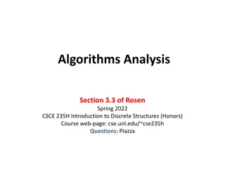
Example: Polynomial Evaluation

600

500

400

300

200

100

35

30

25

20

15

10

5

g(n) = n

T(n) = n

2

/2 + n/2

f(n) = n

2

 # of mult’s

n (degree of polynomial)

13-18

S

u

m

o

f

F

i

r

s

t

n

N

a

t

u

r

a

l

N

u

m

b

e

r

s

Write down the terms of the sum in forward and reverse

orders; there are 

n

 terms:

T(n) =  1 +   2     +   3    + … + (n-2) + (n-1) + n

T(n) =  n + (n-1) + (n-2) + … +   3    +    2    + 1

Add the terms in the boxes to get:

2

*T(n) = (n+1) + (n+1) + (n+1) + … + (n+1) + (n+1) + (n+1)

           = 

n

(n+1)

Therefore, T(n) = (n*(n+1))/2 = n

2

/2 + n/2

13-19

Big-O Notation

•

F

o

r

m

a

l

l

y

,

t

h

e

t

i

m

e

c

o

m

p

l

e

x

i

t

y

T

(

n

)

o

f

a

n

a

l

g

o

r

i

t

h

m

i

s

O

(

f

(

n

)

)

(

o

f

t

h

e

o

r

d

e

r

f

(

n

)

)

i

f

,

f

o

r

s

o

m

e

p

o

s

i

t

i

v

e

c

o

n

s

t

a

n

t

s

C

1

a

n

d

C

2

f

o

r

a

l

l

b

u

t

f

i

n

i

t

e

l

y

m

a

n

y

v

a

l

u

e

s

o

f

n

     C

1

*f(n)   

≤

   T(n)  

≤

   C

2

*f(n)

•

This gives 

upper 

and 

lower bounds

 on the

amount of work done for all sufficiently large 

n

13-20

Big-O Notation

E

x

a

m

p

l

e

:

B

r

u

t

e

f

o

r

c

e

m

e

t

h

o

d

f

o

r

p

o

l

y

n

o

m

i

a

l

e

v

a

l

u

a

t

i

o

n

:

W

e

c

h

o

s

e

t

h

e

h

i

g

h

e

s

t

-

o

r

d

e

r

t

e

r

m

o

f

t

h

e

e

x

p

r

e

s

s

i

o

n

T

(

n

)

=

n

2

/

2

+

n

/

2

,

w

i

t

h

a

c

o

e

f

f

i

c

i

e

n

t

o

f

1

,

s

o

t

h

a

t

f

(

n

)

=

n

2

.

T(n)/n

2

 approaches 

1/2

 for large 

n

, so 

T(n)

 is

approximately 

n

2

/2

.

         n

2

/2 <= T(n) <= n

2

         so 

T(n)

 is 

O(n

2

)

.

13-21

Big-O Notation

•

We want an easily recognized

elementary function to describe the

performance of the algorithm, so we use

the 

dominant term

 of 

T(n)

: it determines

the basic 

shape

 of the function

13-22

Worst Case vs. Average Case

•

Worst case analysis

 is used to find an

upper bound on algorithm performance

for large problems (large 

n

)

•

Average case analysis

 determines the

average (or 

expected

) performance

•

Worst case time complexity is usually

simpler to work out

13-23

Big-O Analysis in General

•

With 

independent

 nested loops: The

number of iterations of the inner loop is

independent of the number of iterations

of the outer loop

•

Example

:

 int x = 0;

 for ( int j = 1; j <= n/2; j++ )

     for ( int k = 1; k <= n*n; k++ )

         x = x + j + k;

Outer loop executes 

n/2

 times.

For each of those times, inner

loop executes 

n

2

 times, so the

body of the inner loop is

executed 

(n/2)*n

2

 = n

3

/2

 times.

The algorithm is 

O(n

3

) 

.

13-24

Big-O Analysis in General

•

With 

dependent

 nested loops: Number

of iterations of the inner loop depends

on a value from the outer loop

•

Example

:

 int x = 0;

 for ( int j = 1; j <= n; j++ )

     for ( int k = 1; k < 3*j; k++ )

         x = x + j;

When 

j

 is 1, inner loop executes 

3

times; when 

j

 is 

2

, inner loop executes

3*2

 times; … when 

j

 is 

n

, inner loop

executes 

3*n

 times. In all the inner loop

executes 

3+6+9+…+3n

 =

3(1+2+3+…+n)

 = 

3n

2

/2 + 3n/2

 times.

The algorithm is 

O(n

2

)

.

13-25

Big-O Analysis in General

Assume that a computer executes a million instructions a second.

This chart summarizes the amount of time required to execute 

f(n)

instructions on this machine for various values of 

n

.

13-26

27

Order-of-Magnitude Analysis

and Big O Notation

F

i

g

u

r

e

9

-

3

a

A

c

o

m

p

a

r

i

s

o

n

o

f

g

r

o

w

t

h

-

r

a

t

e

f

u

n

c

t

i

o

n

s

:

(

a

)

i

n

t

a

b

u

l

a

r

f

o

r

m

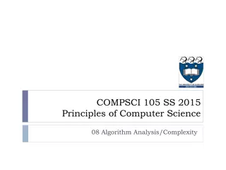
28

Order-of-Magnitude Analysis

and Big O Notation

F

i

g

u

r

e

9

-

3

b

A

c

o

m

p

a

r

i

s

o

n

o

f

g

r

o

w

t

h

-

r

a

t

e

f

u

n

c

t

i

o

n

s

:

(

b

)

i

n

g

r

a

p

h

i

c

a

l

f

o

r

m

Big-O Analysis in General

•

To determine the time complexity of an

algorithm:

•

Express the amount of work done as a

sum 

f

1

(n) + f

2

(n) + … + f

k

(n)

•

Identify the 

dominant term

: the 

f

i

 such that

f

j

is 

O(f

i

)

 and for 

k 

different from

 j

                       f

k

(n) <

f

j

 (n) 

(for all sufficiently large n)

•

Then the time complexity is

 O(f

i

)

13-29

Big-O Analysis in General

•

Examples of 

dominant terms

:

 n dominates log

2

(n)

 n*log

2

(n) dominates n

 n

2

 dominates n*log

2

(n)

 n

m

 dominates n

k

 when m > k

 a

n

 dominates n

m

 for any a > 1 and m >= 0

•

That is, log

2

(n) < n < n*log

2

(n) < n

2

 < …

< n

m

 < a

n

 for a >= 1 and m > 2

13-30

Intractable problems

•

A problem is said to be 

intractable

 if

solving it by computer is impractical

•

E

x

a

m

p

l

e

:

A

l

g

o

r

i

t

h

m

s

w

i

t

h

t

i

m

e

c

o

m

p

l

e

x

i

t

y

O

(

2

n

)

t

a

k

e

t

o

o

l

o

n

g

t

o

s

o

l

v

e

e

v

e

n

f

o

r

m

o

d

e

r

a

t

e

v

a

l

u

e

s

o

f

n

;

a

m

a

c

h

i

n

e

t

h

a

t

e

x

e

c

u

t

e

s

1

0

0

m

i

l

l

i

o

n

i

n

s

t

r

u

c

t

i

o

n

s

p

e

r

s

e

c

o

n

d

c

a

n

e

x

e

c

u

t

e

2

6

0

i

n

s

t

r

u

c

t

i

o

n

s

i

n

a

b

o

u

t

3

6

5

y

e

a

r

s

13-31

•

STOP

32

Constant Time Complexity

•

Algorithms whose solutions are independent

of the size of the problem’s inputs are said

to have 

constant

 time complexity

•

Constant time complexity is denoted as 

O(1)

13-33

Time Complexities for Data Structure

Operations

•

Many operations on the data structures

we’ve seen so far are clearly 

O(1)

:

retrieving the size, testing emptiness, etc

•

We can often recognize the time

complexity of an operation that modifies

the data structure without a formal proof

13-34

Time Complexities for Array

Operations

•

Array elements are stored contiguously

in memory, so the time required to

compute the memory address of an

array element 

arr[k]

 is independent of the

array’s size: It’s the 

start address

of

 arr

plus

 k * (size of an individual element)

•

So, storing and retrieving array elements

are 

O(1)

 operations

13-35

Time Complexities for Array-Based

List Operations

•

Assume an 

n

-element

 List

:

•

insert

 operation is 

O(n)

 in the worst case,

which is adding to the first location: all 

n

elements in the array have to be shifted one

place to the right before the new element can

be added

13-36

Time Complexities for Array-Based

List Operations

•

Inserting into a full 

List

 is also 

O(n)

:

•

replaceContainer

 copies array contents

from the old array to a new one (

O(n)

)

•

All other activies (allocating the new array,

deleting the old one, etc) are 

O(1)

•

Replacing the array and then inserting at

the beginning requires

 O(n) + O(n) 

time,

which is

 O(n)

13-37

Time Complexities for Array-Based

List Operations

•

remove

 operation is 

O(n)

 in the worst case,

which is removing from the first location: 

n-1

array elements must be shifted one place left

•

retrieve

,

 replace

,

 and 

swap

 operations are 

O(1)

:

array indexing allows direct access to an array

location, independent of the array size; no

shifting occurs

•

find

 is 

O(n)

 because the entire list has to be

searched in the worst case

13-38

Time Complexities for Linked List

Operations

•

Singly linked list with 

n

 nodes:

•

addHead

, 

removeHead

, and 

retrieveHead

are all 

O(1)

•

a

d

d

T

a

i

l

a

n

d

r

e

t

r

i

e

v

e

T

a

i

l

a

r

e

O

(

1

)

p

r

o

v

i

d

e

d

t

h

a

t

t

h

e

i

m

p

l

e

m

e

n

t

a

t

i

o

n

h

a

s

a

t

a

i

l

r

e

f

e

r

e

n

c

e

;

o

t

h

e

r

w

i

s

e

,

t

h

e

y

’

r

e

O

(

n

)

•

removeTail

 is 

O(n)

: need to traverse to the

second-last node so that its reference can

be reset to 

NULL

13-39

Time Complexities for Linked List

Operations

•

Singly linked list with 

n

 nodes (cont’d):

•

Operations to access an item by position

(

add 

,

 retrieve

, 

remove(unsigned int k)

,

replace

) are 

O(n)

:

need to traverse the

whole list in the worst case

•

Operations to access an item by its value

(

find

, 

remove(Item item)

) are 

O(n)

 for the

same reason

13-40

Time Complexities for Linked List

Operations

•

Doubly-linked list with 

n

 nodes:

•

S

a

m

e

a

s

f

o

r

s

i

n

g

l

y

-

l

i

n

k

e

d

l

i

s

t

s

,

e

x

c

e

p

t

t

h

a

t

a

l

l

h

e

a

d

a

n

d

t

a

i

l

o

p

e

r

a

t

i

o

n

s

,

i

n

c

l

u

d

i

n

g

r

e

m

o

v

e

T

a

i

l

,

a

r

e

O

(

1

)

•

Ordered linked list with 

n

 nodes:

•

Comparable operations to those found in the linked

list class have the same time complexities

•

add(Item item)

 operation is 

O(n)

: may have to

traverse the whole list

13-41

Time Complexities for Stack

Operations

•

Stack using an underlying array:

•

All operations are 

O(1)

, provided that the

top of the stack is always at the highest

index currently in use: no shifting required

•

Stack using an array-based list:

•

All operations 

O(1)

, provided that the tail of

the list is the top of the stack

•

E

x

c

e

p

t

i

o

n

:

p

u

s

h

i

s

O

(

n

)

i

f

t

h

e

a

r

r

a

y

s

i

z

e

h

a

s

t

o

d

o

u

b

l

e

13-42

Time Complexities for Stack

Operations

•

Stack using an underlying linked list:

•

All operations are, or should be, 

O(1)

•

Top of stack is the head of the linked list

•

If a doubly-linked list with a tail pointer is

used, the top of the stack can be the tail of

the list

13-43

Time Complexities for Queue

Operations

•

Queue using an underlying array-based list:

•

peek

is 

O(1)

•

enqueue

is 

O(1) 

unless the array size has to

be increased (in which case it’s

 O(n)

)

•

dequeue

 is 

O(n)

 : all the remaining elements

have to be shifted

13-44

Time Complexities for Queue

Operations

•

Queue using an underlying linked list:

•

As long as we have both a head and a tail

pointer in the linked list, all operations are 

O(1)

•

important:   

enqueue()

 should use 

addTail()    

dequeue()

 should use 

removeHead()

Why not the other way around?

•

No need for the list to be doubly-linked

13-45

Time Complexities for Queue

Operations

•

Circular queue using an underlying array:

•

All operations are 

O(1)

•

If we revise the code so that the queue can

be arbitrarily large, enqueue is 

O(n)

 on those

occasions when the underlying array has to

be replaced

13-46

Time Complexities for OrderedList

Operations

OrderedList

 with array-based 

m_container

:

•

O

u

r

i

m

p

l

e

m

e

n

t

a

t

i

o

n

o

f

i

n

s

e

r

t

(

i

t

e

m

)

(

s

e

e

s

l

i

d

e

1

0

-

1

2

)

u

s

e

s

“

l

i

n

e

a

r

s

e

a

r

c

h

”

t

h

a

t

t

r

a

v

e

r

s

e

s

t

h

e

l

i

s

t

f

r

o

m

i

t

s

b

e

g

i

n

n

i

n

g

u

n

t

i

l

t

h

e

r

i

g

h

t

s

p

o

t

f

o

r

t

h

e

n

e

w

i

t

e

m

i

s

f

o

u

n

d

–

l

i

n

e

a

r

c

o

m

p

l

e

x

i

t

y

O

(

n

)

•

Operation 

remove(int pos)

is also  

O(n)

 since

items have to be shifted in the array

13-47

Basic Search Algorithms and

their Complexity Analysis

13-48

Linear Search: Example 1

•

The problem

: Search an array 

a

 of size 

n

 to

determine whether the array contains the

value 

key

; return index if found, -1 if not found

 Set 

k

 to 0.

 While (

k

 < 

n

) and (

a[k]

 is not 

key

)

    Add 1 to 

k

.

If  

k 

== 

n  

Return –1.

Return 

k

.

13-49

Analysis of Linear Search

•

Total amount of work done:

•

Before loop: a constant amount 

a

•

Each time through loop: 2 comparisons, an

and

 operation, and an addition: a constant

amount of work 

b

•

After loop: a constant amount 

c

•

In worst case, we examine all

 n 

array

locations, so

 T(n) = a +b*n + c = b*n + d,

where

 d = a+c, 

and

time complexity is

 O(n)

13-50

Analysis of Linear Search

•

Simpler (less formal) analysis:

•

Note that work done before and after loop is

independent of 

n

, and work done during a

single execution of loop is independent of 

n

•

In worst case, loop will be executed 

n

 times,

so amount of work done is proportional to 

n

,

and algorithm is 

O(n)

13-51

Analysis of Linear Search

•

Average

 case for a 

successful

 search:

•

Probability of 

key

 being found at index 

k

 is

1 in n 

for each value of

 k

•

Add up the amount of work done in each

case, and divide by total number of cases:

((a*1+d) + (a*2+d) + (a*3+d) + … + (a*n+d))/n

= (n*d + a*(1+2+3+ … +n))/n

= n*d/n + a*(n*(n+1)/2)/n = d + a*n/2 + a/2 = (a/2)*n + e,

where constant e=d+a/2, so expected case is also 

O(n)

13-52

Analysis of Linear Search

•

Simpler approach to expected case:

•

Add up the number of times the loop is

executed in each of the 

n

 cases, and divide

by the number of cases 

n

•

(1+2+3+ … +(n-1)+n)/n = (n*(n+1)/2)/n =

n/2 + 1/2; algorithm is therefore 

O(n)

13-53

Linear Search for LinkedList

•

Linear search can be also done for 

LinkedList

•

e

x

e

r

c

i

s

e

:

w

r

i

t

e

c

o

d

e

f

o

r

f

u

n

c

t

i

o

n

•

Complexity of function 

find(key)

 for class

LinkedList

 should also be 

O(n)

13-54

t

e

m

p

l

a

t

e

<

c

l

a

s

s

I

t

e

m

>

t

e

m

p

l

a

t

e

<

c

l

a

s

s

E

q

u

a

l

i

t

y

>

i

n

t

L

i

n

k

e

d

L

i

s

t

<

I

t

e

m

>

:

:

f

i

n

d

(

I

t

e

m

k

e

y

)

c

o

n

s

t

{

…

}

 Binary Search

(on sorted arrays)

•

General case: search a sorted array 

a

of size 

n

 looking for the value 

key

•

Divide and conquer

 approach:

•

Compute the middle index 

mid

 of the array

•

If 

key

 is found at 

mid

, we’re done

•

Otherwise repeat the approach on the half

of the array that might still contain 

key

•

etc…

13-55

Example: Binary Search For

Ordered List

int binarySearch(m_container, key)   {

       int first = 1,    last = m_container.getLength();

       while (first <= last) {     

// start of 

while

 loop

             int mid    =  (first+last)/2;

             Item val  =  retrieve(mid);

             if         (key < 

 v

al)     last = mid-1;

             else if  (key >  val)    first = mid+1;

             else                              return  mid;

      }      

// end of 

while

 loop

      return –1;

}

13-56

Analysis of Binary Search

•

The amount of work done before and

after the loop is a constant, and

independent of 

n

•

The amount of work done during a

single execution of the loop is constant

•

Time complexity will therefore be

proportional to number of times the loop

is executed, so that’s what we’ll analyze

13-57

Analysis of Binary Search

•

Worst case

: 

key

 is not found in the array

•

Each time through the loop, at least half

of the remaining locations are rejected:

•

After first time through, 

<= n/2

 remain

•

After second time through, 

<= n/4

 remain

•

After third time through, 

<= n/8

 remain

•

After k

th

 time through, 

<= n/2

k

 remain

13-58

Analysis of Binary Search

•

Suppose in the worst case that maximum

number of times through the loop is 

k

; we

must express 

k

 in terms of 

n

•

Exit the do..while loop when number of

remaining possible locations is less than

1 (that is, when 

first > last

): this means

that 

n/2

k 

< 1

13-59

Analysis of Binary Search

•

Also, 

n/2

k-1

 >=1

; otherwise, looping

would have stopped after 

k-1

 iterations

•

Combining the two inequalities, we get:

n/2

k

 < 1 <= n/2 

k-1

•

Invert and multiply through by 

n

 to get:

2

k

 > n >= 2 

k-1

13-60

Analysis of Binary Search

•

Next, take base-2 logarithms to get:

 k > log

2

(n) >= k-1

•

Which is equivalent to:

 log

2

(n) < k <= log

2

(n) + 1

•

Thus, binary search algorithm is

O(log

2

(n))

 in terms of the number of

array locations examined

13-61

Binary vs. Liner Search

13-62

search

  for one 

out of 

n

ordered integers

see demo: 

www.csd.uwo.ca/courses/CS1037a/demos.html

n

t

t

n

Basic Sorting Algorithms and

their Complexity Analysis

13-63

Analysis: Selection Sort Algorithm

•

Assume we have an unsorted collection

of 

n

 elements in an array or list called

container

; elements are either of a

simple type, or are pointers to data

•

Assume that the elements can be

compared in size ( 

<

, 

>

, 

==

,

etc

)

•

Sorting will take place

“in place”

in

container

13-64

6

4

9

2

3

2

4

9

6

3

2

4

9

6

3

Find smallest element in unsorted

portion of 

container

Interchange the smallest element with the

one at the front of the unsorted portion

Find smallest element in unsorted

portion of 

container

2

3

9

6

4

Interchange the smallest element with the

one at the front of the unsorted portion

Analysis: Selection Sort Algorithm

- sorted portion of the list

- minimum element in unsorted portion

13-65

Analysis: Selection Sort Algorithm

2

3

9

6

4

Find smallest element in unsorted

portion of 

container

2

3

9

4

6

Interchange the smallest element with the

one at the front of the unsorted portion

2

3

9

4

6

Find smallest element in unsorted

portion of 

container

2

3

6

4

9

Interchange the smallest element with the

one at the front of the unsorted portion

A

f

t

e

r

n

-

1

r

e

p

e

t

i

t

i

o

n

s

o

f

t

h

i

s

p

r

o

c

e

s

s

,

t

h

e

l

a

s

t

i

t

e

m

h

a

s

a

u

t

o

m

a

t

i

c

a

l

l

y

f

a

l

l

e

n

i

n

t

o

p

l

a

c

e

- sorted portion of the list

- minimum element in unsorted portion

13-66

Selection Sort for

(array-based) List

v

o

i

d

s

e

l

e

c

t

i

o

n

S

o

r

t

(

l

i

s

t

,

i

t

e

m

s

)

{

u

n

s

i

g

n

e

d

i

n

t

m

i

n

S

o

F

a

r

,

i

,

k

;

f

o

r

(

i

=

1

;

i

<

i

t

e

m

s

;

i

+

+

)

{

/

/

‘

u

n

s

o

r

t

e

d

’

p

a

r

t

s

t

a

r

t

s

a

t

g

i

v

e

n

‘

i

’

m

i

n

S

o

F

a

r

=

i

;

f

o

r

(

k

=

i

+

1

;

k

<

=

i

t

e

m

s

;

k

+

+

)

/

/

s

e

a

r

c

h

i

n

g

f

o

r

m

i

n

I

t

e

m

i

n

s

i

d

e

‘

u

n

s

o

r

t

e

d

’

i

f

(

l

i

s

t

[

k

]

<

l

i

s

t

[

m

i

n

S

o

F

a

r

]

)

m

i

n

S

o

F

a

r

=

k

;

s

w

a

p

(

l

i

s

t

[

i

]

,

l

i

s

t

[

m

i

n

S

o

F

a

r

]

)

;

}

/

/

e

n

d

o

f

f

o

r

-

i

l

o

o

p

}

// A new member function for class List<Item>, needs additional template parameter

13-67

Analysis: Selection Sort Algorithm

•

We’ll determine the time complexity for

selection sort by counting the number of

data items examined in sorting an 

n

-

item array or list

•

Outer loop is executed 

n-1

 times

•

Each time through the outer loop, one

more item is sorted into position

13-68

Analysis: Selection Sort Algorithm

•

On the 

k

th

 time through the outer loop:

•

Sorted portion of 

container

 holds 

k-1

 items

initially, and unsorted portion holds 

n-k+1

•

Position of the first of these is saved in

minSoFar

; data object is not examined

•

In the inner loop, the remaining 

n-k

 items

are compared  to the one at 

minSoFar

 to

decide if 

minSoFar

 has to be reset

13-69

Analysis: Selection Sort Algorithm

•

2

 data objects are examined each time

through the inner loop

•

So, in total, 

2*(n-k)

 data objects are

examined by the inner loop during the 

k

th

pass through the outer loop

•

Two elements may be switched

following the inner loop, but the data

values aren’t examined (compared)

13-70

Analysis: Selection Sort Algorithm

•

Overall, on the 

k

th

 time through the

outer loop, 

2*(n-k)

 objects are examined

•

But 

k

 ranges from 

1

 to 

n-1

 (the number

of times through the outer loop)

•

Total number of elements examined is:

T

(

n

)

=

2

*

(

n

-

1

)

+

2

*

(

n

-

2

)

+

2

*

(

n

-

3

)

+

…

+

2

*

(

n

-

(

n

-

2

)

)

+

2

*

(

n

-

(

n

-

1

)

)

        = 2*((n-1) + (n-2) + (n-3) + … + 2 + 1) 

(or 2*(sum of first n-1 ints)

=

2

*

(

(

n

-

1

)

*

n

)

/

2

)

=

n

2

–

n

,

s

o

t

h

e

a

l

g

o

r

i

t

h

m

i

s

O

(

n

2

)

13-71

Analysis: Selection Sort Algorithm

•

This analysis works for both arrays and

array-based lists, provided that, in the

list implementation, we either directly

access array 

m_container

, or use

retrieve

 and 

replace

 operations 

(

O(1)

operations)

 rather than 

insert

 and 

remove

(

O(n) 

operations)

72

Analysis: Selection Sort Algorithm

•

The algorithm has 

deterministic

  complexity

-

the number of operations does not depend on

specific items, it depends only on the number of

items

-

a

l

l

p

o

s

s

i

b

l

e

i

n

s

t

a

n

c

e

s

o

f

t

h

e

p

r

o

b

l

e

m

(

“

b

e

s

t

c

a

s

e

”

,

“

w

o

r

s

t

c

a

s

e

”

,

“

a

v

e

r

a

g

e

c

a

s

e

”

)

g

i

v

e

t

h

e

s

a

m

e

n

u

m

b

e

r

o

f

o

p

e

r

a

t

i

o

n

s

T

(

n

)

=

n

2

–

n

=

O

(

n

2

)

13-73

Radix Sort

•

Sorts objects based on some 

key

 value

found within the object

•

Most often used when keys are strings

of the same length, or positive integers

with the same number of digits

•

Uses queues; does not sort “in place”

•

Other names: 

postal

, 

bin, bucket sort

13-74

Radix Sort Algorithm

•

Suppose keys are 

k-digit

 integers

•

Radix sort uses an array of 10 queues, one

for each digit 0 through 9

•

Each object is placed into the queue whose

index is the least significant digit (the 1’s digit)

of the object’s key

•

Objects are then dequeued from these 10

queues, in order 0 through 9, and put back in

the original queue/list/array container; they’re

sorted by the last digit of the key

13-75

Radix Sort Algorithm

•

Process is repeated, this time using the 10’s digit

instead of the 1’s digit; values are now sorted by

last two digits of the key

•

Keep repeating, using the 100’s digit, then the

1000’s digit, then the 10000’s digit, …

•

Stop after using the most significant (10

n-1

’s ) digit

•

Objects are now in order in original container

13-76

Algorithm

: Radix Sort

 Assume 

n

 items to be sorted, 

k

 digits per key, and 

t 

possible values

 for a digit of a key, 

0

 through 

t-1

. (

k

 and 

t

 are constants.)

 For each of the 

k

 digits in a key:

     While the queue 

q

 is not empty:

         Dequeue an element 

e

 from 

q

.

         Isolate the 

k

th

digit from the right in the key for 

e

; call it 

d

.

         Enqueue 

e

 in the 

d

th

 queue in the array of queues 

arr

.

    For each of the 

t

 queues in 

arr

:

         While 

arr[t-1]

 is not empty

             Dequeue an element from 

arr[t-1]

 and enqueue it in 

q

.

13-77

Radix Sort Example

Suppose keys are 4-digit numbers using only the digits 0, 1, 2

and 3, and that we wish to sort the following queue of objects

whose keys are shown:

3023

1030

2222

1322

3100

1133

2310

13-78

Radix Sort Example

302

3

103

0

222

2

132

2

310

0

113

3

231

0

0

1

2

3

.

Array of queues after

the 

first

pass

103

0

310

0

231

0

222

2

132

2

302

3

113

3

Then, items are moved back to the original queue (first all items from the top

queue, then from the 2

nd

, 3

rd

, and the bottom one):

3023

1030

2222

1322

3100

1133

2310

First

 pass: while the queue above is not empty, dequeue an item and add it

    into one of the queues below based on the item’s last digit

13-79

Radix Sort Example

30

2

3

10

3

0

22

2

2

13

2

2

31

0

0

11

3

3

23

1

0

Array of queues after

the 

second

 pass

10

30

31

00

23

10

22

22

13

22

30

23

11

33

103

0

310

0

231

0

222

2

132

2

302

3

113

3

0

1

2

3

Second

 pass: while the queue above is not empty, dequeue an item and

add it into one of the queues below based on the item’s 2

nd

 last digit

Then, items are moved back to the original queue (first all items from the top

queue, then from the 2

nd

, 3

rd

, and the bottom one):

13-80

Radix Sort Example

3

0

23

1

0

30

2

2

22

1

3

22

3

1

00

1

1

33

2

3

10

Array of queues after

the 

third

 pass

1

030

3

100

2

310

2

222

1

322

3

023

1

133

10

30

31

00

23

10

22

22

13

22

30

23

11

33

0

1

2

3

First

 pass: while the queue above is not empty, dequeue an item and add it

    into one of the queues below based on the item’s 3

rd

 last digit

Then, items are moved back to the original queue (first all items from the top

queue, then from the 2

nd

, 3

rd

, and the bottom one):

13-81

Radix Sort Example

3

023

1

030

2

222

1

322

3

100

1

133

2

310

Array of queues after

the

fourth

 pass

1030

3100

2310

2222

1322

3023

1133

.

1

030

3

100

2

310

2

222

1

322

3

023

1

133

0

1

2

3

First

 pass: while the queue above is not empty, dequeue an item and add it

    into one of the queues below based on the item’s first digit

Then, items are moved back to the original queue (first all items from the top

queue, then from the 2

nd

, 3

rd

, and the bottom one):      

NOW IN ORDER

13-82

Analysis: Radix Sort

•

We’ll count the total number of enqueue

and dequeue operations

•

Each time through the outer 

for

 loop:

•

In the 

while

 loop: 

n

 elements are dequeued

from 

q

 and enqueued somewhere in 

arr

: 

2*n

operations

•

In the inner 

for

 loop: a total of 

n

 elements

are dequeued from queues in 

arr

 and

enqueued in 

q

: 

2*n

 operations

13-83

Analysis: Radix Sort

•

So, we perform 

4*n

 enqueue and dequeue

operations each time through the outer loop

•

Outer for loop is executed 

k

 times, so we have

4*k*n

 enqueue and dequeue operations

altogether

•

But 

k

 is a constant, so the time complexity for

radix sort is 

O(n)

•

COMMENT: If the maximum number of digits in

each number 

k

 is considered as a parameter

describing problem input, then complexity can be

written in general as

 O(n*k) 

or

 O(n*log(max_val))

13-84