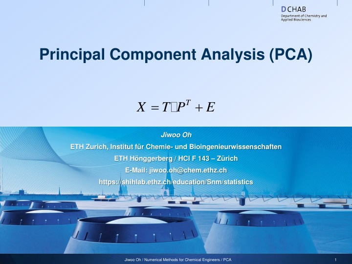
Principal Component Analysis (PCA)
Principal Component Analysis (PCA) is a statistical method used to analyze high-dimensional data matrices. It involves finding the principal components that best represent the data points in a lower-dimensional space. The process includes geometric interpretations such as representing data points in X-space, determining the first principal component line, adding orthogonal principal components to form a plane, projecting data onto this plane, and summarizing variables through scores and loadings. PCA is a valuable tool for visualizing data and identifying important variables in chemical and biotechnological processes.

Download Presentation

Please find below an Image/Link to download the presentation.
The content on the website is provided AS IS for your information and personal use only. It may not be sold, licensed, or shared on other websites without obtaining consent from the author.If you encounter any issues during the download, it is possible that the publisher has removed the file from their server.
You are allowed to download the files provided on this website for personal or commercial use, subject to the condition that they are used lawfully. All files are the property of their respective owners.
The content on the website is provided AS IS for your information and personal use only. It may not be sold, licensed, or shared on other websites without obtaining consent from the author.
E N D
Presentation Transcript
Principal Component Analysis (PCA) = + T X T P E Jiwoo Oh ETH Zurich, Institut f r Chemie- und Bioingenieurwissenschaften ETH H nggerberg / HCI F 143 Z rich E-Mail: jiwoo.oh@chem.ethz.ch https://shihlab.ethz.ch/education/Snm/statistics Jiwoo Oh / Numerical Methods for Chemical Engineers / PCA 1
Geometric interpretation: Average Each row or object in X is represented by one point in X- space. The data matrix X represents a swarm of points in this space. The vector of variable averages is also a point in X-space. This average is then subtracted from the data matrix. This corresponds to moving the origin of the coordinate system to the middle ( center-of- mass ) of the data swarm. X3 X2 X1 Jiwoo Oh / Numerical Methods for Chemical Engineers / PCA 2
Geometric interpretation: 1. Principal Component (PC) The first principal component (PC) is a line in X-space that best approximates the data (in the least squares sense). It explains the greatest possible amount of variation. The line goes through the average point. The direction of the line is determined by the loading vector p1(elements p1k). The position of each point, is determined by the score vector t1 (elements t1i) Linear transformation and projection X3 X2 X1 Jiwoo Oh / Numerical Methods for Chemical Engineers / PCA 3
Geometric interpretation: PC-plane New orthogonal PCs can be added improving the approximation of the data points as much as possible. The principal components together form a plane (hyperplane) in X- space.The line goes through the average point. PCA is a visualization tool projecting the data points onto a low dimensional plane. This allows considering the (process) data from a window (television analogy) of representative non- correlated (latent) variables. X3 X2 X1 Jiwoo Oh / Numerical Methods for Chemical Engineers / PCA 4
Geometric interpretation: Projection The scores t are a small number of new variables (latent variables) that best summarize the original ones. Sorted on importance: t1, t2,.. The values of the latent variables for each object are called scores tia (component a and object i) Scores are the locations along the lines where the objects are projected. The loadings p define the orientation of the lines. Computation through NIPALS algorithm (Nonlinear Iterative Partial Least Squares) Jiwoo Oh / Numerical Methods for Chemical Engineers / PCA 5
PCA: Residuals Information Noise Jiwoo Oh / Numerical Methods for Chemical Engineers / PCA 6
Why PCA? Chemical and Biotechnological Process data: Very high dimensional data matrices Many variables and many observations Variables are not independent High correlation among variables Low signal to noise ratio Each variable contains little information need multivariate methods Separation of information from noise Main effects are captured by the first PCs while the rest can be attributed to noise Non-causal in nature Can t generally use data to imply cause and effect relationships But can get informative correlation relationships (exploration, description) Biotechnology: very limited mathematical (first principle law) understanding of interactions between the large amount of variables Jiwoo Oh / Numerical Methods for Chemical Engineers / PCA 7
p2 Information from PCA Score plots (e.g. t1 vs t2) Observation groups Abnormal behavior (outliers) Loading plots (e.g. p1 vs p2) Correlation of variables Importance of variables (to explain overall X-variance) Hotelling s T2 plot Distance of point from the origin in the plane. How different is it from average condition? SPE (sum of projection error) plot Distance of point from plane. Which objects p1 Jiwoo Oh / Numerical Methods for Chemical Engineers / PCA 8
PCA: Food example Jiwoo Oh / Numerical Methods for Chemical Engineers / PCA 9
PCA: Food example score plot (t1, t2) Jiwoo Oh / Numerical Methods for Chemical Engineers / PCA 10
PCA: Food example loading plot (p1, p2) correlated Negatively correlated to green group Not correlated to green group Jiwoo Oh / Numerical Methods for Chemical Engineers / PCA 11
PCA: Food example combination Loadings and Scores are unidirectional Jiwoo Oh / Numerical Methods for Chemical Engineers / PCA 12
PCA: Food example abnormal behavior from SPE plot Far from plane Close to plane Jiwoo Oh / Numerical Methods for Chemical Engineers / PCA 13
PCA: Wine example Loadings Scores Jiwoo Oh / Numerical Methods for Chemical Engineers / PCA 14
PCA: Writer example Scores + Loadings Jiwoo Oh / Numerical Methods for Chemical Engineers / PCA 15
PCA in Matlab Use the following set of functions for PCA: [loadings,scores,varexp,tsquare] = princomp(Z) Performs PCA on standardized X-data set Outputs: loadings, scores, variance explained by each PC and Hoteling's T2 distance [loadings,scores,vexpZ,tsquared,vexpX,mu] = pca(Z) Performs PCA on standardized X-data set Outputs: loadings, scores, variance explained by each PC in X and Z, Hoteling's T2 distance, estimated mean of each variable in X biplot(loadings(:,1:3),'scores',scores(:,1:3),'varlabels',vbls); Plots the loadings and scores in a single plot Z = zscore(X) Standardizes the raw X-matrix Jiwoo Oh / Numerical Methods for Chemical Engineers / PCA 16
Exercise 12 One of the first multivariate data sets was introduced by Sir Ronald Fisher in 1936. This data quantifies the morphologic variation of Iris flowers of three related species. Jiwoo Oh / Numerical Methods for Chemical Engineers / PCA 17
Assignment 1 1. Read in the data set Fisher Iris.xlsx 2. Standardize the four numeric X variables. 3. Perform a Principal Component Analysis using the function princomp on the standardized data. 4. Plot the specific and cumulative variance explained by the principal components normalizing it by the maximal variance explained, s.t. R2max = 1. What can you interpret regarding the general correlation structure of the variables? How many main effects seem to be present in the data? 5. Plot the loadings and scores of the first two principal components with biplot. Can you observe different groups? Distinguish those groups by showing the different flower species in different colors and labeling them with their species name using text an additional scatter plot. What can you conclude regarding the correlation of the variables and the main effects in the data? Jiwoo Oh / Numerical Methods for Chemical Engineers / PCA 18
Assignment 1 (Continued) 6. Consider the correlation matrix (using the function corrcoef) to support your first conclusion. 7. Which species features most of the abnormal observations? Use the Hotelling s T2 distance in the plane of the first two PCs (t1 and t2) for each observation i comparing it to a critical value of 6.3 (corresponds to 95 % level). Using the variances of t1 and t2, s12 and s22, it can be defined as 8. Which species can be worst explained by the model with two PCs? How could you improve this deviation from the model plane? Calculate the SPE value for each observation comparing it to critical level of 0.6 (corresponds to 95 % level). You can access the residuals using the function pcares. 9. Re-perform the analysis without the standardization step. Which changes do you observe? Why? Jiwoo Oh / Numerical Methods for Chemical Engineers / PCA 19
")

")


")
")


")