Phylogenetic Analysis and Tree Terminology
Phylogenetics is the study of evolutionary history using tree diagrams to represent organism pedigrees. Analyzing fossil records, molecular data, DNA sequence evolution, and tree terminology play crucial roles. Understanding dichotomy vs. polytomy, rooted vs. unrooted trees, and the challenges of finding a correct tree topology with branch lengths are essential in phylogenetic analysis.

Download Presentation

Please find below an Image/Link to download the presentation.
The content on the website is provided AS IS for your information and personal use only. It may not be sold, licensed, or shared on other websites without obtaining consent from the author.If you encounter any issues during the download, it is possible that the publisher has removed the file from their server.
You are allowed to download the files provided on this website for personal or commercial use, subject to the condition that they are used lawfully. All files are the property of their respective owners.
The content on the website is provided AS IS for your information and personal use only. It may not be sold, licensed, or shared on other websites without obtaining consent from the author.
E N D
Presentation Transcript
PHYLOGENETIC ANALYSIS
Phylogenetics Phylogenetics is the study of the evolutionary history of living organisms using treelike diagrams to represent pedigrees of these organisms. The tree branching patterns representing the evolutionary divergence are referred to as phylogeny.
http://www.agiweb.org/news/evolution/fossilrecord.html Studying phylogenetics Fossil records morphological information, available only for certain species, data can be fragmentary, morphological traits are ambiguous, fossil record nonexistent for microorganisms Molecular data (molecular fossils) more numerous than fossils, easier to obtain, favorite for reconstruction of the evolutionary history
Tree of life http://tikalon.com/blog/blog.php?article=2011/domains
DNA sequence evolution AAGACTT -3 mil yrs -2 mil yrs AAGGCCT AAGGCCT TGGACTT TGGACTT AGGGCAT TAGCCCT AGCACTT -1 mil yrs today AGGGCAT TAGCCCA TAGACTT AGCACAA AGCGCTT www.cs.utexas.edu/users/tandy/CSBtutorial.ppt
Tree terminology Terminal nodes taxa (taxon) Branches A B C D Ancestral node or root of the tree E Internal nodes or Divergence points (represent hypothetical ancestors of the taxa) Based on lectures by Tal Pupko
dichotomy all branches bifurcate, vs. polytomy result of a taxon giving rise to more than two descendants or unresolved phylogeny (the exact order of bifurcations can not be determined exactly)
unrooted no knowledge of a common ancestor, shows relative relationship of taxa, no direction of an evolutionary path rooted obviously, more informative
Finding a true tree is difficult Correct reconstruction of the evolutionary history = find a correct tree topology with correct branch lengths. Number of potential tree topologies can be enormously large even with a moderate number of taxa. 2? 3 ! 2? 2? 2 ! ??= 2? 5 ! 2? 3? 3 ! ??= 6 taxa NR = 945, NU = 105 10 taxa NR = 34 459 425, NU= 2 027 025
Rooting the tree B C To root a tree mentally, imagine that the tree is made of string. Grab the string at the root and tug on it until the ends of the string (the taxa) fall opposite the root: Root D Unrooted tree A A C B D Note that in this rooted tree, taxon A is no more closely related to taxon B than it is to C or D. Rooted tree Root Based on lectures by Tal Pupko
Now, try it again with the root at another position: B C Root Unrooted tree D A A B C D Rooted tree Note that in this rooted tree, taxon A is most closely related to taxon B, and together they are equally distantly related to taxa C and D. Root Based on lectures by Tal Pupko
An unrooted, four-taxon tree theoretically can be rooted in five different places to produce five different rooted trees 2 4 A C The unrooted tree 1: 1 5 D B 3 Rooted tree 1a Rooted tree 1b Rooted tree 1c Rooted tree 1d Rooted tree 1e B A A C D A B D C B C C C A A D B B D D These trees show five different evolutionary relationships among the taxa! Based on lectures by Tal Pupko
Rooting the tree outgroup taxa (the outgroup ) that are known to fall outside of the group of interest (the ingroup ). Requires some prior knowledge about the relationships among the taxa. The outgroup can either be species (e.g., birds to root a mammalian tree) or previous gene duplicates (e.g., -globins to root -globins). outgroup Based on lectures by Tal Pupko
Rooting the tree midpoint rooting approach - roots the tree at the midway point between the two most distant taxa in the tree, as determined by branch lengths. Assumes that the taxa are evolving in a clock-like manner. A d (A,D) = 10 + 3 + 5 = 18 Midpoint = 18 / 2 = 9 10 C 3 2 2 B D 5 Based on lectures by Tal Pupko
Molecular clock This concept was proposed by Emil Zuckerkandl and Linus Pauling (1962) as well as by Emanuel Margoliash (1963). For every given gene (or protein), the rate of molecular evolution is approximately constant. Pioneering study by Zuckerkandl and Pauling They observed the number of amino acid differences between human globins and (~ 6 differences), and (~ 36 differences), and (~ 78 differences), and and (~ 83 differences). They could also compare human to gorilla (both and globins), observing either 2 or 1 differences respectively. They knew from fossil evidence that humans and gorillas diverged from a common ancestor about 11 MYA. Using this divergence time as a calibration point, they estimated that gene duplications of the common ancestor to and occurred 44 MYA; and derived from a common ancestor 260MYA; and 565 MYA; and and 600MYA.
Gene phylogeny vs. species phylogeny Main objective of building phylogenetic trees based on molecular sequences: reconstruct the evolutionary history of the species involved. A gene phylogeny only describes the evolution of that particular gene or encoded protein. This sequence may evolve more or less rapidly than other genes in the genome. The evolution of a particular sequence does not necessarily correlate with the evolutionary path of the species. Branching point in a species tree the speciation event Branching point in a gene tree which event? The two events may or may not coincide. To obtain a species phylogeny, phylogenetic trees from a variety of gene families need to be constructed to give an overall assessment of the species evolution.
Closest living relatives of humans? Based on lectures by Tal Pupko
Closest living relatives of humans? Humans Gorillas Chimpanzees Chimpanzees Bonobos Bonobos Gorillas Orangutans Orangutans Humans 14 0 0 15-30 MYA MYA The pre-molecular view was that the great apes (chimpanzees, gorillas and orangutans) formed a clade separate from humans, and that humans diverged from the apes at least 15-30 MYA. Mitochondrial DNA, most nuclear DNA- encoded genes, and DNA/DNA hybridization all show that bonobos and chimpanzees are related more closely to humans than to gorillas.
Orangutan Human Gorilla Chimpanzee From the Tree of the Life Website, University of Arizona
Forms of tree representation phylogram branch lengths represent the amount of evolutionary divergence cladogram external taxa line up neatly, only the topology matters
Taxon B Taxon C No meaning to the spacing between the taxa, or to the order in which they appear from top to bottom. Taxon A Taxon D Taxon E This dimension either can have no scale (for cladograms ), can be proportional to genetic distance or amount of change (for phylograms ), or can be proportional to time (for ultrametric trees or true evolutionary trees). ((A,(B,C)),(D,E)) = The above phylogeny as nested parentheses These say that B and C are more closely related to each other than either is to A, and that A, B, and C form a clade that is a sister group to the clade composed of D and E. If the tree has a time scale, then D and E are the most closely related. Based on lectures by Tal Pupko
Procedure 1. Choice of molecular markers 2. Multiple sequence alignment 3. Choice of a model of evolution 4. Determine a tree building method 5. Assess tree reliability
Choice of molecular markers Nucleotide or protein sequence data? NA sequences evolve more rapidly. They can be used for studying very closely related organisms. E. g., for evolutionary analysis of different individuals within a population, noncoding regions of mtDNA are often used. Evolution of more divergent organisms either slowly evolving NA (e.g., rRNA) or protein sequences. Deepest level (e.g., relatioships between bacteria and eukaryotes) conserved protein sequences
MSA Critical step Multiple state-of-the-art alignment programs (e.g., T- Coffee, Praline, Poa, ) should be used. The alignment results from multiple sources should be inspected and compared carefully to identify the most reasonable one. Automatic sequence alignments almost always contain errors and should be further edited or refined if necessary manual editing! Rascal and NorMD can help to improve alignment by correcting alignment errors and removing potentially unrelated or highly divergent sequences.
Model of evolution A simple measure of the divergence of two sequences number of substitutions in the alignment, a distance between two sequences a proportion of substitutions If A was replaced by C: A C or A T G C? Back mutation: G C G. Parallel mutations both sequences mutate into e.g., T at the same time. All of this obscures the estimation of the true evolutionary distances between sequences. This effect is known as homoplasy and must be corrected. Statistical models infer the true evolutionary distances between sequences.
Transition: YY, RR Transversion: YR, RY Model of evolution Homplasy is corrected by substitution (evolutionary) models. There exists a lot of such models. Jukes-Cantor model ???= 3 4 ?? 1 4 3 ??? dAB distance, pAB proportion of substitutions example: alignment of A and B is 20 nucleotides long, 6 pairs are different, pAB= 0.3, dAB= 0.38 Kimura model ???= 1 2 ?? 1 2??? ??? 1 4 ln(1 2???) pti frequency of transition, ptv frequency of transversion
Models of amino acids substitutions use the amino acid substitution matrix PAM JTT 90s, the same methodology as PAM, but with larger protein database protein equivalents of of Jukes Cantor and Kimura models, e.g., ? = ln(1 ? 0.2 ?2)
Among site variations Up to now we have assumed that different positions in a sequence are assumed to be evolving at the same rate. However, in reality this may not be true. In DNA, the rates of substitution differ for different codon positions. 3rdcodon mutates much faster. In proteins, some AAs change rarely than others owing to functional constraints. It has been shown that there are always a proportion of positions in a sequence dataset that have invariant rates and a proportion that have more variable rates.
To account for site-dependent rate variation, a correction factor ? is used. ? is derived from statistics. For the Jukes Cantor model, the evolution distance can be adjusted with the following formula: 1 ???= (3/4)?[ 1 4 ? 1] 3 ??? For the Kimura model, the evolutionary distance becomes ? 2 1 2 1 1 ???= 1 2??? ??? ? 1 2??? ? 1/2]
Tree building methods Two major categories. Distance based methods. Based on the amount of dissimilarity between pairs of sequences, computed on the basis of sequence alignment. Characters based methods. Based on discrete characters, which are molecular sequences from individual taxa.
Tree building methods COMPUTATIONAL METHOD Optimality criterion Clustering algorithm Characters Maximum parsimony (MP) Maximum likelihood (ML) DATA TYPE Fitch-Margoliash (FM) UPGMA Distances Neighbor-joining (NJ)
Distance based methods Calculate evolutionary distances dABbetween sequences using some of the evolutionary model. Construct a distance matrix distances between all pairs of taxa. Based on the distance scores, construct a phylogenetic tree. clustering algorithms UPGMA, neighbor joining (NJ) optimality based Fitch-Margoliash (FM)
Clustering methods UPGMA (Unweighted Pair Group Method with Arithmetic Mean) Hierachical clustering, agglomerative, you know it as an average linkage Produces rooted tree (most phylogenetic methods produce unrooted tree). Basic assumption of the UPGMA method: all taxa evolve at a constant rate, they are equally distant from the root, implying that a molecular clock is in effect. However, real data rarely meet this assumption. Thus, UPGMA often produces erroneous tree topologies.
Neighbor joining A 0 B 2 0 C 3 3 0 D 4 4 3 0 E 4 5 4 5 0 C A B C D E A D E A,B C D E B C A,B 0 2.5 4.5 3.5 C 0 D E A 3 0 4 5 0 D A,B B E C A The Minimum Evolution (ME) criterion: in each iteration we separate the two sequences which result with the minimal sum of branch lengths D E B
Distance based pros and cons clustering Fast, can handle large datasets Not guaranteed to find the best tree UPGMA assumes a constant rate of evolution of the sequences in all branches of the tree (molecular clock assumption) NJ does not assume that the rate of evolution is the same in all branches of the tree NJ is slower but better than UPGMA exhaustive tree searching (Fitch-Margoliash) better accuracy, prohibitive for more than 12 taxa
Character based methods Also called discrete methods Based directly on the sequence characters They count mutational events accumulated on the sequences and may therefore avoid the loss of information when characters are converted to distances. Evolutionary dynamics of each character can be studied The two most popular character-based approaches: maximum parsimony (MP) and maximum likelihood (ML) methods.
Maximum parsimony Based on Occam s razor. William of Occam, 13thcentury. The simplest explanation is probably the correct one. This is because the simplest explanation requires the fewest assumptions and the fewest leaps of logic. A tree with the least number of substitutions is probably the best to explain the differences among the taxa under study.
A worked example 1 A A A A 2 A G G G 3 G C A A 4 A C T G 5 G G A A 6 T T T T 7 G G C C 8 C C C C 9 A G A G 1 2 3 4 To save computing time, only a small number of sites that have the richest phylogenetic information are used in tree determination. informative site sites that have at least two different kinds of characters, each occurring at least twice
A worked example 1 A A A A 2 A G G G 3 G C A A 4 A C T G 5 G G A A 6 T T T T 7 G G C C 8 C C C C 9 A G A G 1 2 3 4 To save computing time, only a small number of sites that have the richest phylogenetic information are used in tree determination. informative site sites that have at least two different kinds of characters, each occurring at least twice
How many possible unrooted trees? 1 G G A A 2 G G C C 3 A G A G 1 2 3 4 2? 5 ! 2? 3? 3 ! ??= 1 1 1 3 2 3 2 3 4 4 4 2 Tree I Tree II Tree III
GGAA G A A G G G 3 1 A G G G 4 2 Tree I A A G A 3 1 Tree II G G 4 2 2 1 G A Tree III 4 3
GGCC G C C G G G C G G G Tree I C C G C Tree II G G G C Tree III
AGAG A A A A A G G G G A Tree I G A A A Tree II G G G G Tree III
I II 2 2 1 5 III 2 2 2 6 1 1 2 4 GGAA GGCC AGAG Tree length ACA GGA ACA GGA 2 1 1 GGG ACG Tree I
Weighted parsimony The parsimony method discussed so far is unweighted because it treats all mutations as equivalent. This may be an oversimplification; mutations of some sites are known to occur less frequently than others, for example, transversions versus transitions, functionally important sites versus neutral sites. A weighting scheme takes into account the different kinds of mutations.
Branch-and-bound The parsimony method examines all possible tree topologies to find the maximally parsimonious tree. This is an exhaustive search method, expensive. N = 10 2 027 025 N = 20 2.22 1020 Branch-and-bound Rationale: a maximally parsimonious tree must be equal to or shorter than the distance-based tree. First build a distance tree using NJ or UPGMA. Compute the minimum number of substitutions for this tree. The resulting number defines the upper bound to which any other trees are compared. I.e., when you build a parsimonous tree, you stop growing it when its length exceeds the upper bound.
Heuristic methods When a number of taxa exceeds 20, even branch-and- bound becomes computationally unfeasible. Then, heuristic search can be applied. Both exhaustive search and branch-and-bound methods lead to the optimum tree. Heuristic search leads to the suboptimum tree (compare to BLAST which is also heuristic).