Perceptron Learning Algorithm in Neural Networks


CS 270 - Perceptron
1

CS 270 - Perceptron
2
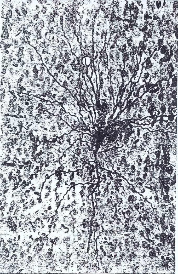
Basic Neuron
CS 270 - Perceptron
3
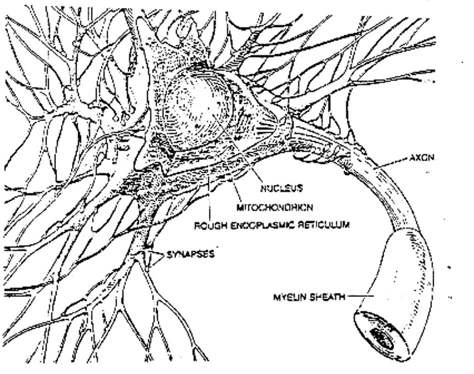
Expanded Neuron
CS 270 - Perceptron
4
Perceptron Learning Algorithm
First neural network learning model in the 1960’s
–
Frank Rosenblatt
Simple and limited (single layer model)
Basic concepts are similar for multi-layer models so this is
a good learning tool
Still used in some current applications (large business
problems, where intelligibility is needed, etc.)
CS 270 - Perceptron
5
Perceptron Node – Threshold Logic Unit
x
1
x
n
x
2
w
1
w
2
w
n
z
CS 270 - Perceptron
6
Perceptron Node – Threshold Logic Unit
x
1
x
n
x
2
w
1
w
2
w
n
z
•
Learn weights such that an objective
function is maximized.
•
What objective function should we use?
•
What learning algorithm should we use?
CS 270 - Perceptron
7
Perceptron Learning Algorithm
x
1
x
2
z
.4
-.2
.1
CS 270 - Perceptron
8
First Training Instance
z
.4
-.2
.1
net
= .8*.4 + .3*-.2 = .26
=1
CS 270 - Perceptron
9
Second Training Instance
z
.4
-.2
.1
net
= .4*.4 + .1*-.2 = .14
=1
w
i
=
t - z
c
x
i
CS 270 - Perceptron
10
Perceptron Rule Learning
w
i
= c
t – z
)
x
i
Where
w
i
is the weight from input
i
to the perceptron node,
c
is the
learning rate,
t
is the target for the current instance,
z
is the current output,
and
x
i
is
i
th
input
Least perturbation principle
–
Only change weights if there is an error
–
small
c
rather than changing weights sufficient to make current pattern correct
–
Scale by
x
i
Create a perceptron node with
n
inputs
Iteratively apply a pattern from the training set and apply the perceptron
rule
Each iteration through the training set is an
epoch
Continue training until total training set error ceases to improve
Perceptron Convergence Theorem: Guaranteed to find a solution in finite
time if a solution exists
CS 270 - Perceptron
11
CS 270 - Perceptron
12
Augmented Pattern Vectors
1 0 1 -> 0
1 0 0 -> 1
Augmented Version
1 0 1 1 -> 0
1 0 0 1 -> 1
Treat threshold like any other weight. No special case.
Call it a
bias
since it biases the output up or down.
Since we start with random weights anyways, can ignore
the -
notion, and just think of the bias as an extra
available weight. (note the author uses a -1 input)
Always use a bias weight
CS 270 - Perceptron
13
Perceptron Rule Example
Assume a 3 input perceptron plus bias (it outputs 1 if net > 0, else 0)
Assume a learning rate
c
of 1 and initial weights all 0:
w
i
= c
t – z
)
x
i
Training set
0 0 1 -> 0
1 1 1 -> 1
1 0 1 -> 1
0 1 1 -> 0
Pattern
Target (
t
)
Weight Vector (
w
i
)
Net
Output (
z
)
W
0 0 1 1
0
0 0 0 0
CS 270 - Perceptron
14
Example
Assume a 3 input perceptron plus bias (it outputs 1 if net > 0, else 0)
Assume a learning rate
c
of 1 and initial weights all 0:
w
i
= c
t – z
)
x
i
Training set
0 0 1 -> 0
1 1 1 -> 1
1 0 1 -> 1
0 1 1 -> 0
Pattern
Target (
t
)
Weight Vector (
w
i
)
Net
Output (
z
)
W
0 0 1 1
0
0 0 0 0
0
0
0 0 0 0
1 1 1 1
1
0 0 0 0
CS 270 - Perceptron
15
Example
Assume a 3 input perceptron plus bias (it outputs 1 if net > 0, else 0)
Assume a learning rate
c
of 1 and initial weights all 0:
w
i
= c
t – z
)
x
i
Training set
0 0 1 -> 0
1 1 1 -> 1
1 0 1 -> 1
0 1 1 -> 0
Pattern
Target (
t
)
Weight Vector (
w
i
)
Net
Output (
z
)
W
0 0 1 1
0
0 0 0 0
0
0
0 0 0 0
1 1 1 1
1
0 0 0 0
0
0
1 1 1 1
1 0 1 1
1
1 1 1 1
Peer Instruction
I pose a
challenge question
(often multiple choice), which
will help solidify understanding of topics we have studied
–
Might not just be one correct answer
You each get some time (1-2 minutes) to come up with
your answer and vote
–
use Mentimeter (anonymous)
Then you get some time to convince your group
(neighbors) why you think you are right (2-3 minutes)
–
Learn from and teach each other
!
You vote again. May change your vote if you want.
We discuss together the different responses, show the
votes, give you opportunity to justify your thinking, and
give you further insights
CS 270 - Perceptron
16
Peer Instruction (PI) Why
Studies show this approach
improves learning
Learn by doing, discussing, and teaching each other
–
Curse of knowledge/expert blind-spot
–
Compared to talking with a peer who just figured it out and who can
explain it in your own jargon
–
You never really know something until you can teach it to someone
else
–
More improved learning!
Learn to reason about your thinking and answers
More enjoyable - You are involved and active in the learning
CS 270 - Perceptron
17
How Groups Interact
Best if group members have different initial answers
3 is the “magic” group number
–
You can self-organize "on-the-fly" or sit together specifically to be a
group
–
Can go 2-4 on a given day to make sure everyone is involved
Teach and learn from each other: Discuss, reason, articulate
If you know the answer, listen to where colleagues are coming
from first, then be a great humble teacher, you will also learn by
doing that, and you’ll be on the other side in the future
–
I can’t do that as well because every small group has different
misunderstandings and you get to focus on your particular questions
Be ready to justify to the class your vote and justifications!
CS 270 - Perceptron
18
CS 270 - Perceptron
19
**Challenge Question** - Perceptron
Assume a 3 input perceptron plus bias (it outputs 1 if net > 0, else 0)
Assume a learning rate
c
of 1 and initial weights all 0:
w
i
= c
t – z
)
x
i
Training set
0 0 1 -> 0
1 1 1 -> 1
1 0 1 -> 1
0 1 1 -> 0
Pattern
Target (
t
)
Weight Vector (
w
i
)
Net
Output (
z
)
W
0 0 1 1
0
0 0 0 0
0
0
0 0 0 0
1 1 1 1
1
0 0 0 0
0
0
1 1 1 1
1 0 1 1
1
1 1 1 1
Once it converges the final weight vector will be
A.
1 1 1 1
B.
-1 0 1 0
C.
0 0 0 0
D.
1 0 0 0
E.
None of the above
CS 270 - Perceptron
20
Example
Assume a 3 input perceptron plus bias (it outputs 1 if net > 0, else 0)
Assume a learning rate
c
of 1 and initial weights all 0:
w
i
= c
t – z
)
x
i
Training set
0 0 1 -> 0
1 1 1 -> 1
1 0 1 -> 1
0 1 1 -> 0
Pattern
Target (
t
)
Weight Vector (
w
i
)
Net
Output (
z
)
W
0 0 1 1
0
0 0 0 0
0
0
0 0 0 0
1 1 1 1
1
0 0 0 0
0
0
1 1 1 1
1 0 1 1
1
1 1 1 1
3
1
0 0 0 0
0 1 1 1
0
1 1 1 1
CS 270 - Perceptron
21
Example
Assume a 3 input perceptron plus bias (it outputs 1 if net > 0, else 0)
Assume a learning rate
c
of 1 and initial weights all 0:
w
i
= c
t – z
)
x
i
Training set
0 0 1 -> 0
1 1 1 -> 1
1 0 1 -> 1
0 1 1 -> 0
Pattern
Target (
t
)
Weight Vector (
w
i
)
Net
Output (
z
)
W
0 0 1 1
0
0 0 0 0
0
0
0 0 0 0
1 1 1 1
1
0 0 0 0
0
0
1 1 1 1
1 0 1 1
1
1 1 1 1
3
1
0 0 0 0
0 1 1 1
0
1 1 1 1
3
1
0 -1 -1 -1
0 0 1 1
0
1 0 0 0
CS 270 - Perceptron
22
Example
Assume a 3 input perceptron plus bias (it outputs 1 if net > 0, else 0)
Assume a learning rate
c
of 1 and initial weights all 0:
w
i
= c
t – z
)
x
i
Training set
0 0 1 -> 0
1 1 1 -> 1
1 0 1 -> 1
0 1 1 -> 0
Pattern
Target (
t
)
Weight Vector (
w
i
)
Net
Output (
z
)
W
0 0 1 1
0
0 0 0 0
0
0
0 0 0 0
1 1 1 1
1
0 0 0 0
0
0
1 1 1 1
1 0 1 1
1
1 1 1 1
3
1
0 0 0 0
0 1 1 1
0
1 1 1 1
3
1
0 -1 -1 -1
0 0 1 1
0
1 0 0 0
0
0
0 0 0 0
1 1 1 1
1
1 0 0 0
1
1
0 0 0 0
1 0 1 1
1
1 0 0 0
1
1
0 0 0 0
0 1 1 1
0
1 0 0 0
0
0
0 0 0 0
CS 270 - Perceptron
23
Perceptron Homework
Assume a 3 input perceptron plus bias (it outputs 1 if net > 0, else 0)
Assume a learning rate
c
of 1 and initial weights all 1:
w
i
= c
t – z
)
x
i
Show weights after each pattern for just one epoch
Training set
1 0 1 -> 0
1 .5 0 -> 0
1 -.4 1 -> 1
0 1 .5 -> 1
Pattern
Target (
t
)
Weight Vector (
w
i
)
Net
Output (
z
)
W
1 1 1 1
CS 270 - Perceptron
24
Training Sets and Noise
Assume a Probability of Error at each input and output
value each time a pattern is trained on
0 0 1 0 1 1 0 0 1 1 0 -> 0 1 1 0
i.e. P(error) = .05
Or a probability that the algorithm is applied wrong
(opposite) occasionally
Averages out over learning
CS 270 - Perceptron
25
CS 270 - Perceptron
26
If no bias weight, the
hyperplane must go
through the origin.
Note that since 𝛳 = -bias,
the equation with bias is:
X
2
=
(
-W
1
/W
2
)
X
1
- bias/W
2
CS 270 - Perceptron
27
Linear Separability
CS 270 - Perceptron
28
Linear Separability and Generalization
When is data noise vs. a legitimate exception
CS 270 - Perceptron
29
Limited Functionality of Hyperplane
How to Handle Multi-Class Output
This is an issue with learning models which only support binary
classification (perceptron, SVM, etc.)
Create 1 perceptron for each output class, where the training set
considers all other classes to be negative examples (one vs the
rest)
–
Run all perceptrons on novel data and set the output to the class of the
perceptron which outputs high
–
If there is a tie, choose the perceptron with the highest net value
Another approach: Create 1 perceptron for each pair of output
classes, where the training set only contains examples from the
2 classes (one vs one)
–
Run all perceptrons on novel data and set the output to be the class
with the most wins (votes) from the perceptrons
–
In case of a tie, use the net values to decide
–
Number of models grows by the square of the output classes
CS 270 - Perceptron
30
CS 270 - Perceptron
31
UC Irvine Machine Learning Data Base
Iris Data Set
4.8,3.0,1.4,0.3,
Iris-setosa
5.1,3.8,1.6,0.2,
Iris-setosa
4.6,3.2,1.4,0.2,
Iris-setosa
5.3,3.7,1.5,0.2,
Iris-setosa
5.0,3.3,1.4,0.2,
Iris-setosa
7.0,3.2,4.7,1.4,
Iris-versicolor
6.4,3.2,4.5,1.5,
Iris-versicolor
6.9,3.1,4.9,1.5,
Iris-versicolor
5.5,2.3,4.0,1.3,
Iris-versicolor
6.5,2.8,4.6,1.5,
Iris-versicolor
6.0,2.2,5.0,1.5,
Iris-viginica
6.9,3.2,5.7,2.3,
Iris-viginica
5.6,2.8,4.9,2.0,
Iris-viginica
7.7,2.8,6.7,2.0,
Iris-viginica
6.3,2.7,4.9,1.8,
Iris-viginica
Objective Functions: Accuracy/Error
How do we judge the quality of a particular model (e.g.
Perceptron with a particular setting of weights)
Consider how accurate the model is on the data set
–
Classification accuracy
= # Correct/Total instances
–
Classification error
= # Misclassified/Total instances (= 1 – acc)
Usually minimize a Loss function (aka cost, error)
For real valued outputs and/or targets
–
Pattern error = Target – output: Errors could cancel each other
|
t
j
– z
j
| (L1 loss)
where
j
indexes all outputs in the pattern
Common approach is
Squared Error
=
(
t
j
– z
j
)
2
(L2 loss)
–
Total sum squared error =
pattern squared errors =
(
t
ij
– z
ij
)
2
where
i
indexes all the patterns in training set
For nominal data, pattern error is typically 1 for a mismatch and
0 for a match
–
For nominal (including binary) output and targets, L!, L2, and
classification error are equivalent
CS 270 - Perceptron
32
Mean Squared Error
Mean Squared Error (MSE) – SSE/
n
where
n
is the number of
instances in the data set
–
This can be nice because it normalizes the error for data sets of
different sizes
–
MSE is the average squared error per pattern
Root Mean Squared Error (RMSE) – is the square root of the
MSE
–
This puts the error value back into the same units as the features and
can thus be more intuitive
Since we squared the error on the SSE
–
RMSE is the average distance (error) of targets from the outputs in the
same scale as the features
–
Note RMSE is the root of the total data set MSE, and NOT the sum of
the root of each individual pattern MSE
CS 270 - Perceptron
33
**Challenge Question** - Error
Given the following data set, what is the L1 (
|
t
i
– z
i
|), SSE (L2)
(
(
t
i
– z
i
)
2
), MSE, and RMSE error for the entire data set?
CS 270 - Perceptron
34
A.
.4 1 1 1
B.
1.6 2.36 1 1
C.
.4 .64 .21 0.453
D.
1.6 1.36 .67 .82
E.
None of the above
**Challenge Question** - Error
CS 270 - Perceptron
35
A.
.4 1 1 1
B.
1.6 2.36 1 1
C.
.4 .64 .21 0.453
D.
1.6 1.36 .67 .82
E.
None of the above
Given the following data set, what is the L1 (
|
t
i
– z
i
|), SSE (L2)
(
(
t
i
– z
i
)
2
), MSE, and RMSE error for the entire data set?
Error Values Homework
Given the following data set, what is the L1, SSE (L2), MSE,
and RMSE error of Output1, Output2, and the entire data set?
Fill in cells that have a ?.
–
Notes: For instance 1 the L1 pattern error is 1 + .6 = 1.6 and the SSE
pattern error is 1 + .16 = 1.16. The Data Set L1 and SSE errors will
just be the sum of each of the pattern errors.
CS 270 - Perceptron
36
CS 270 - Perceptron
37
Gradient Descent Learning: Minimize
(Maximize) the Objective Function
Total SSE:
Sum
Squared
Error
(
t – z
)
2
0
Error Landscape
Weight Values
CS 270 - Perceptron
38
Goal is to decrease overall error (or other loss function)
each time a weight is changed
Total Sum Squared error one possible loss function
E
:
(
t – z
)
2
Seek a weight changing algorithm such that is
negative
If a formula can be found then we have a gradient descent
learning algorithm
Delta rule is a variant of the perceptron rule which gives a
gradient descent learning algorithm with perceptron nodes
Deriving a Gradient Descent Learning
Algorithm
CS 270 - Perceptron
39
Delta rule algorithm
Delta rule uses (target - net) before the net value goes through the
threshold in the learning rule to decide weight update
Weights are updated even when the output would be correct
Because this model is single layer and because of the SSE objective
function, the error surface is guaranteed to be parabolic with only one
minima
Learning rate
–
If learning rate is too large can jump around global minimum
–
If too small, will get to minimum, but will take a longer time
–
Can decrease learning rate over time to give higher speed and still
attain the global minimum (although exact minimum is still just for
training set and thus…)
Batch vs Stochastic Update
To get the true gradient with the delta rule, we need to sum
errors over the entire training set and only update weights
at the end of each epoch
Batch (gradient) vs stochastic (on-line, incremental)
–
SGD (Stochastic Gradient Descent)
–
With the stochastic delta rule algorithm, you update after every pattern,
just like with the perceptron algorithm (even though that means each
change may not be along the true gradient)
–
Stochastic is more efficient and best to use in almost all cases, though not
all have figured it out yet
–
We’ll talk about this in more detail when we get to Backpropagation
CS 270 - Perceptron
40
CS 270 - Perceptron
41
Perceptron rule vs Delta rule
Perceptron rule (target - thresholded output) guaranteed to
converge to a separating hyperplane if the problem is
linearly separable. Otherwise may not converge – could
get in a cycle
Singe layer Delta rule guaranteed to have only one global
minimum. Thus, it will converge to the best SSE solution
whether the problem is linearly separable or not.
–
Could have a higher misclassification rate than with the perceptron
rule and a less intuitive decision surface – we will discuss this later
with regression where Delta rules is more appropriate
Stopping Criteria – For these models we stop when no
longer making progress
–
When you have gone a few epochs with no significant
improvement/change between epochs (including oscillations)
CS 270 - Perceptron
42
CS 270 - Perceptron
43
Linearly Separable Boolean Functions
d
= # of dimensions (i.e. inputs)
CS 270 - Perceptron
44
Linearly Separable Boolean Functions
d
= # of dimensions
P = 2
d
= # of Patterns
CS 270 - Perceptron
45
Linearly Separable Boolean Functions
d
= # of dimensions
P = 2
d
= # of Patterns
2
P
=
2
2
d
= # of Functions
n
Total Functions
Linearly Separable Functions
0
2
2
1
4
4
2
16
14
CS 270 - Perceptron
46
Linearly Separable Boolean Functions
d
= # of dimensions
P = 2
d
= # of Patterns
2
P
=
2
2
d
= # of Functions
n
Total Functions
Linearly Separable Functions
0
2
2
1
4
4
2
16
14
3
256
104
4
65536
1882
5
4.3 × 10
9
94572
6
1.8 × 10
19
1.5 × 10
7
7
3.4 × 10
38
8.4 × 10
9
CS 270 - Perceptron
47
Linear Models which are Non-Linear in the
Input Space
So far we have used
We could preprocess the inputs in a non-linear way and do
To the perceptron algorithm it is the same but with
more/different inputs. It still uses the same learning algorithm.
For example, for a problem with two inputs
x
and
y
(plus the
bias), we could also add the inputs
x
2
,
y
2
, and
x
·
y
The perceptron would just think it is a 5-dimensional task, and it
is linear (5-d hyperplane) in those 5 dimensions
–
But what kind of decision surfaces would it allow for the original 2-
d
input space?
CS 270 - Perceptron
48
Quadric Machine
All quadratic surfaces (2
nd
order)
–
ellipsoid
–
parabola
–
etc.
That significantly increases the number of problems that
can be solved
Can we solve XOR with this setup?
CS 270 - Perceptron
49
Quadric Machine
All quadratic surfaces (2
nd
order)
–
ellipsoid
–
parabola
–
etc.
That significantly increases the number of problems that
can be solved
But still many problem which are not quadrically separable
Could go to 3
rd
and higher order features, but number of
possible features grows exponentially
Multi-layer neural networks will allow us to discover high-
order features automatically from the input space
CS 270 - Perceptron
50
Simple Quadric Example
What is the decision surface for a 1-d (1 input) problem?
Perceptron with just feature
f
1
cannot separate the data
Could we add a transformed feature to our perceptron?
CS 270 - Perceptron
51
-3 -2 -1 0 1 2 3
f
1
Simple Quadric Example
Perceptron with just feature
f
1
cannot separate the data
Could we add a transformed feature to our perceptron?
f
2
=
f
1
2
CS 270 - Perceptron
52
-3 -2 -1 0 1 2 3
f
1
Simple Quadric Example
Perceptron with just feature
f
1
cannot separate the data
Could we add another feature to our perceptron
f
2
=
f
1
2
Note could also think of this as just using feature
f
1
but now
allowing a quadric surface to divide the data
–
Note that
f
1
not actually needed in this case
CS 270 - Perceptron
53
-3 -2 -1 0 1 2 3
f
1
-3 -2 -1 0 1 2 3
f
2
f
1
Quadric Machine Homework
Assume a 2-input perceptron expanded to be a quadric (2
nd
order)
perceptron, with 5 input weights (
x
,
y
,
x
·
y
,
x
2
,
y
2
) and the bias weight
–
Assume it outputs 1 if net > 0, else 0
Assume a learning rate
c
of .5 and initial weights all 0
–
w
i
= c
t – z
)
x
i
Show all weights after each pattern for one epoch with
the following
training set
CS 270 - Perceptron
54
Put up Mentimeter at beginning of class for them to sign on
Perceptron is the first neural network learning model introduced in the 1960s by Frank Rosenblatt. It follows a simple and limited (single-layer model) approach but shares basic concepts with multi-layer models. Perceptron is still used in some current applications, especially in large business problems where intelligibility is crucial. The learning process involves adjusting weights to maximize an objective function, with specific rules dictating how weights are updated based on the input data. By iteratively applying patterns from the training set and following the perceptron rule, the algorithm learns to make predictions based on input features.

Download Presentation

Please find below an Image/Link to download the presentation.
The content on the website is provided AS IS for your information and personal use only. It may not be sold, licensed, or shared on other websites without obtaining consent from the author.If you encounter any issues during the download, it is possible that the publisher has removed the file from their server.
You are allowed to download the files provided on this website for personal or commercial use, subject to the condition that they are used lawfully. All files are the property of their respective owners.
The content on the website is provided AS IS for your information and personal use only. It may not be sold, licensed, or shared on other websites without obtaining consent from the author.
E N D
Presentation Transcript
Basic Neuron CS 270 - Perceptron 2
Expanded Neuron CS 270 - Perceptron 3
Perceptron Learning Algorithm First neural network learning model in the 1960 s Frank Rosenblatt Simple and limited (single layer model) Basic concepts are similar for multi-layer models so this is a good learning tool Still used in some current applications (large business problems, where intelligibility is needed, etc.) CS 270 - Perceptron 4
Perceptron Node Threshold Logic Unit x1 w1 q ? z x2 w2 xn wn n = n q 1 if x w i i 1 i = z = i < q 0 if x w i i 1 CS 270 - Perceptron 5
Perceptron Node Threshold Logic Unit x1 w1 z x2 w2 ? xn wn n = n q 1 if x w Learn weights such that an objective function is maximized. What objective function should we use? What learning algorithm should we use? i i 1 i = z = i < q 0 if x w i i 1 CS 270 - Perceptron 6
Perceptron Learning Algorithm x1 .4 z .1 -.2 x2 n x1 x2 t .3 .4 = n q 1 if x w i i .8 1 1 i = z = i .1 0 < q 0 if x w i i 1 CS 270 - Perceptron 7
First Training Instance .8 .4 z =1 .1 .3 -.2 net = .8*.4 + .3*-.2 = .26 n x1 x2 t .3 .4 = n q 1 if x w i i .8 1 1 i = z = i .1 0 < q 0 if x w i i 1 CS 270 - Perceptron 8
Second Training Instance .4 .4 z =1 .1 .1 -.2 net = .4*.4 + .1*-.2 = .14 n x1 x2 t .3 .4 = n q 1 if x w i i wi =(t - z) c xi .8 1 1 i = z = i .1 0 < q 0 if x w i i 1 CS 270 - Perceptron 9
Perceptron Rule Learning wi = c(t z)xi Where wi is the weight from input i to the perceptron node, c is the learning rate, t is the target for the current instance, z is the current output, and xi is ith input Least perturbation principle Only change weights if there is an error small c rather than changing weights sufficient to make current pattern correct Scale by xi Create a perceptron node with n inputs Iteratively apply a pattern from the training set and apply the perceptron rule Each iteration through the training set is an epoch Continue training until total training set error ceases to improve Perceptron Convergence Theorem: Guaranteed to find a solution in finite time if a solution exists CS 270 - Perceptron 10
Augmented Pattern Vectors 1 0 1 -> 0 1 0 0 -> 1 Augmented Version 1 0 1 1 -> 0 1 0 0 1 -> 1 Treat threshold like any other weight. No special case. Call it a bias since it biases the output up or down. Since we start with random weights anyways, can ignore the - notion, and just think of the bias as an extra available weight. (note the author uses a -1 input) Always use a bias weight CS 270 - Perceptron 12
Perceptron Rule Example Assume a 3 input perceptron plus bias (it outputs 1 if net > 0, else 0) Assume a learning rate c of 1 and initial weights all 0: wi = c(t z)xi Training set 0 0 1 -> 0 1 1 1 -> 1 1 0 1 -> 1 0 1 1 -> 0 Output (z) W Pattern 0 0 1 1 Target (t) Weight Vector (wi) 0 0 0 0 0 Net CS 270 - Perceptron 13
Example Assume a 3 input perceptron plus bias (it outputs 1 if net > 0, else 0) Assume a learning rate c of 1 and initial weights all 0: wi = c(t z)xi Training set 0 0 1 -> 0 1 1 1 -> 1 1 0 1 -> 1 0 1 1 -> 0 Output (z) W 0 Pattern 0 0 1 1 1 1 1 1 Target (t) Weight Vector (wi) 0 0 0 0 0 1 0 0 0 0 Net 0 0 0 0 0 CS 270 - Perceptron 14
Example Assume a 3 input perceptron plus bias (it outputs 1 if net > 0, else 0) Assume a learning rate c of 1 and initial weights all 0: wi = c(t z)xi Training set 0 0 1 -> 0 1 1 1 -> 1 1 0 1 -> 1 0 1 1 -> 0 Output (z) W 0 0 Pattern 0 0 1 1 1 1 1 1 1 0 1 1 Target (t) Weight Vector (wi) 0 0 0 0 0 1 0 0 0 0 1 1 1 1 1 Net 0 0 0 0 0 0 1 1 1 1 CS 270 - Perceptron 15
Peer Instruction I pose a challenge question (often multiple choice), which will help solidify understanding of topics we have studied Might not just be one correct answer You each get some time (1-2 minutes) to come up with your answer and vote use Mentimeter (anonymous) Then you get some time to convince your group (neighbors) why you think you are right (2-3 minutes) Learn from and teach each other! You vote again. May change your vote if you want. We discuss together the different responses, show the votes, give you opportunity to justify your thinking, and give you further insights CS 270 - Perceptron 16
Peer Instruction (PI) Why Studies show this approach improves learning Learn by doing, discussing, and teaching each other Curse of knowledge/expert blind-spot Compared to talking with a peer who just figured it out and who can explain it in your own jargon You never really know something until you can teach it to someone else More improved learning! Learn to reason about your thinking and answers More enjoyable - You are involved and active in the learning CS 270 - Perceptron 17
How Groups Interact Best if group members have different initial answers 3 is the magic group number You can self-organize "on-the-fly" or sit together specifically to be a group Can go 2-4 on a given day to make sure everyone is involved Teach and learn from each other: Discuss, reason, articulate If you know the answer, listen to where colleagues are coming from first, then be a great humble teacher, you will also learn by doing that, and you ll be on the other side in the future I can t do that as well because every small group has different misunderstandings and you get to focus on your particular questions Be ready to justify to the class your vote and justifications! CS 270 - Perceptron 18
**Challenge Question** - Perceptron Assume a 3 input perceptron plus bias (it outputs 1 if net > 0, else 0) Assume a learning rate c of 1 and initial weights all 0: wi = c(t z)xi Training set 0 0 1 -> 0 1 1 1 -> 1 1 0 1 -> 1 0 1 1 -> 0 Output (z) W 0 0 Pattern 0 0 1 1 1 1 1 1 1 0 1 1 Target (t) Weight Vector (wi) 0 0 0 0 0 1 0 0 0 0 1 1 1 1 1 Net 0 0 0 0 0 0 1 1 1 1 Once it converges the final weight vector will be A. 1 1 1 1 B. -1 0 1 0 C. 0 0 0 0 D. 1 0 0 0 E. None of the above CS 270 - Perceptron 19
Example Assume a 3 input perceptron plus bias (it outputs 1 if net > 0, else 0) Assume a learning rate c of 1 and initial weights all 0: wi = c(t z)xi Training set 0 0 1 -> 0 1 1 1 -> 1 1 0 1 -> 1 0 1 1 -> 0 Output (z) W 0 0 1 Pattern 0 0 1 1 1 1 1 1 1 0 1 1 0 1 1 1 Target (t) Weight Vector (wi) 0 0 0 0 0 1 0 0 0 0 1 1 1 1 1 0 1 1 1 1 Net 0 0 3 0 0 0 0 1 1 1 1 0 0 0 0 CS 270 - Perceptron 20
Example Assume a 3 input perceptron plus bias (it outputs 1 if net > 0, else 0) Assume a learning rate c of 1 and initial weights all 0: wi = c(t z)xi Training set 0 0 1 -> 0 1 1 1 -> 1 1 0 1 -> 1 0 1 1 -> 0 Output (z) W 0 0 1 1 Pattern 0 0 1 1 1 1 1 1 1 0 1 1 0 1 1 1 0 0 1 1 Target (t) Weight Vector (wi) 0 0 0 0 0 1 0 0 0 0 1 1 1 1 1 0 1 1 1 1 0 1 0 0 0 Net 0 0 3 3 0 0 0 0 1 1 1 1 0 0 0 0 0 -1 -1 -1 CS 270 - Perceptron 21
Example Assume a 3 input perceptron plus bias (it outputs 1 if net > 0, else 0) Assume a learning rate c of 1 and initial weights all 0: wi = c(t z)xi Training set 0 0 1 -> 0 1 1 1 -> 1 1 0 1 -> 1 0 1 1 -> 0 Output (z) W 0 0 1 1 0 1 1 0 Pattern 0 0 1 1 1 1 1 1 1 0 1 1 0 1 1 1 0 0 1 1 1 1 1 1 1 0 1 1 0 1 1 1 Target (t) Weight Vector (wi) 0 0 0 0 0 1 0 0 0 0 1 1 1 1 1 0 1 1 1 1 0 1 0 0 0 1 1 0 0 0 1 1 0 0 0 0 1 0 0 0 Net 0 0 3 3 0 1 1 0 0 0 0 0 1 1 1 1 0 0 0 0 0 -1 -1 -1 0 0 0 0 0 0 0 0 0 0 0 0 0 0 0 0 CS 270 - Perceptron 22
Perceptron Homework Assume a 3 input perceptron plus bias (it outputs 1 if net > 0, else 0) Assume a learning rate c of 1 and initial weights all 1: wi = c(t z)xi Show weights after each pattern for just one epoch Training set 1 0 1 -> 0 1 .5 0 -> 0 1 -.4 1 -> 1 0 1 .5 -> 1 Output (z) W Pattern Target (t) Weight Vector (wi) 1 1 1 1 Net CS 270 - Perceptron 23
Training Sets and Noise Assume a Probability of Error at each input and output value each time a pattern is trained on 0 0 1 0 1 1 0 0 1 1 0 -> 0 1 1 0 i.e. P(error) = .05 Or a probability that the algorithm is applied wrong (opposite) occasionally Averages out over learning CS 270 - Perceptron 24
If no bias weight, the hyperplane must go through the origin. Note that since ? = -bias, the equation with bias is: X2 = (-W1/W2)X1 - bias/W2 CS 270 - Perceptron 26
Linear Separability CS 270 - Perceptron 27
Linear Separability and Generalization When is data noise vs. a legitimate exception CS 270 - Perceptron 28
Limited Functionality of Hyperplane CS 270 - Perceptron 29
How to Handle Multi-Class Output This is an issue with learning models which only support binary classification (perceptron, SVM, etc.) Create 1 perceptron for each output class, where the training set considers all other classes to be negative examples (one vs the rest) Run all perceptrons on novel data and set the output to the class of the perceptron which outputs high If there is a tie, choose the perceptron with the highest net value Another approach: Create 1 perceptron for each pair of output classes, where the training set only contains examples from the 2 classes (one vs one) Run all perceptrons on novel data and set the output to be the class with the most wins (votes) from the perceptrons In case of a tie, use the net values to decide Number of models grows by the square of the output classes CS 270 - Perceptron 30
UC Irvine Machine Learning Data Base Iris Data Set 4.8,3.0,1.4,0.3, 5.1,3.8,1.6,0.2, 4.6,3.2,1.4,0.2, 5.3,3.7,1.5,0.2, 5.0,3.3,1.4,0.2, 7.0,3.2,4.7,1.4, 6.4,3.2,4.5,1.5, 6.9,3.1,4.9,1.5, 5.5,2.3,4.0,1.3, 6.5,2.8,4.6,1.5, 6.0,2.2,5.0,1.5, 6.9,3.2,5.7,2.3, 5.6,2.8,4.9,2.0, 7.7,2.8,6.7,2.0, 6.3,2.7,4.9,1.8, Iris-setosa Iris-setosa Iris-setosa Iris-setosa Iris-setosa Iris-versicolor Iris-versicolor Iris-versicolor Iris-versicolor Iris-versicolor Iris-viginica Iris-viginica Iris-viginica Iris-viginica Iris-viginica CS 270 - Perceptron 31
Objective Functions: Accuracy/Error How do we judge the quality of a particular model (e.g. Perceptron with a particular setting of weights) Consider how accurate the model is on the data set Classification accuracy = # Correct/Total instances Classification error = # Misclassified/Total instances (= 1 acc) Usually minimize a Loss function (aka cost, error) For real valued outputs and/or targets Pattern error = Target output: Errors could cancel each other |tj zj| (L1 loss) where j indexes all outputs in the pattern Common approach is Squared Error = (tj zj)2 (L2 loss) Total sum squared error = pattern squared errors = (tij zij)2 where i indexes all the patterns in training set For nominal data, pattern error is typically 1 for a mismatch and 0 for a match For nominal (including binary) output and targets, L!, L2, and classification error are equivalent CS 270 - Perceptron 32
Mean Squared Error Mean Squared Error (MSE) SSE/n where n is the number of instances in the data set This can be nice because it normalizes the error for data sets of different sizes MSE is the average squared error per pattern Root Mean Squared Error (RMSE) is the square root of the MSE This puts the error value back into the same units as the features and can thus be more intuitive Since we squared the error on the SSE RMSE is the average distance (error) of targets from the outputs in the same scale as the features Note RMSE is the root of the total data set MSE, and NOT the sum of the root of each individual pattern MSE CS 270 - Perceptron 33
**Challenge Question** - Error Given the following data set, what is the L1 ( |ti zi|), SSE (L2) ( (ti zi)2), MSE, and RMSE error for the entire data set? x y Output Target Data Set 2 -3 1 1 0 1 0 1 .5 .6 .8 .2 L1 ? SSE ? MSE ? RMSE ? .4 1 1 1 1.6 2.36 1 1 .4 .64 .21 0.453 1.6 1.36 .67 .82 None of the above A. B. C. D. E. CS 270 - Perceptron 34
**Challenge Question** - Error Given the following data set, what is the L1 ( |ti zi|), SSE (L2) ( (ti zi)2), MSE, and RMSE error for the entire data set? x y Output Target Data Set 2 -3 1 1 0 1 0 1 .5 .6 .8 .2 L1 1.6 SSE 1.36 MSE 1.36/3 = .453 RMSE .45^.5 = .67 .4 1 1 1 1.6 2.36 1 1 .4 .64 .21 0.453 1.6 1.36 .67 .82 None of the above A. B. C. D. E. CS 270 - Perceptron 35
Error Values Homework Given the following data set, what is the L1, SSE (L2), MSE, and RMSE error of Output1, Output2, and the entire data set? Fill in cells that have a ?. Notes: For instance 1 the L1 pattern error is 1 + .6 = 1.6 and the SSE pattern error is 1 + .16 = 1.16. The Data Set L1 and SSE errors will just be the sum of each of the pattern errors. Instance x y Output1 Target1 Output2 Target 2 Data Set 1 -1 -1 0 1 .6 1.0 2 -1 1 1 1 -.3 0 3 1 -1 1 0 1.2 .5 4 1 1 0 0 0 -.2 L1 ? ? ? SSE ? ? ? MSE ? ? ? RMSE ? ? ? CS 270 - Perceptron 36
Gradient Descent Learning: Minimize (Maximize) the Objective Function Error Landscape Total SSE: Sum Squared Error (t z)2 0 Weight Values CS 270 - Perceptron 37
Deriving a Gradient Descent Learning Algorithm Goal is to decrease overall error (or other loss function) each time a weight is changed Total Sum Squared error one possible loss function E: (t z)2 Seek a weight changing algorithm such that is negative If a formula can be found then we have a gradient descent learning algorithm Delta rule is a variant of the perceptron rule which gives a gradient descent learning algorithm with perceptron nodes E w ij CS 270 - Perceptron 38
Delta rule algorithm Delta rule uses (target - net) before the net value goes through the threshold in the learning rule to decide weight update Dwi=c(t-net)xi Weights are updated even when the output would be correct Because this model is single layer and because of the SSE objective function, the error surface is guaranteed to be parabolic with only one minima Learning rate If learning rate is too large can jump around global minimum If too small, will get to minimum, but will take a longer time Can decrease learning rate over time to give higher speed and still attain the global minimum (although exact minimum is still just for training set and thus ) CS 270 - Perceptron 39
Batch vs Stochastic Update To get the true gradient with the delta rule, we need to sum errors over the entire training set and only update weights at the end of each epoch Batch (gradient) vs stochastic (on-line, incremental) SGD (Stochastic Gradient Descent) With the stochastic delta rule algorithm, you update after every pattern, just like with the perceptron algorithm (even though that means each change may not be along the true gradient) Stochastic is more efficient and best to use in almost all cases, though not all have figured it out yet We ll talk about this in more detail when we get to Backpropagation CS 270 - Perceptron 40
Perceptron rule vs Delta rule Perceptron rule (target - thresholded output) guaranteed to converge to a separating hyperplane if the problem is linearly separable. Otherwise may not converge could get in a cycle Singe layer Delta rule guaranteed to have only one global minimum. Thus, it will converge to the best SSE solution whether the problem is linearly separable or not. Could have a higher misclassification rate than with the perceptron rule and a less intuitive decision surface we will discuss this later with regression where Delta rules is more appropriate Stopping Criteria For these models we stop when no longer making progress When you have gone a few epochs with no significant improvement/change between epochs (including oscillations) CS 270 - Perceptron 41
Exclusive Or 1 0 X2 0 1 X1 Is there a dividing hyperplane? CS 270 - Perceptron 42
Linearly Separable Boolean Functions d = # of dimensions (i.e. inputs) CS 270 - Perceptron 43
Linearly Separable Boolean Functions d = # of dimensions P = 2d = # of Patterns CS 270 - Perceptron 44
Linearly Separable Boolean Functions d = # of dimensions P = 2d = # of Patterns 2P = 22d= # of Functions n Total Functions Linearly Separable Functions 0 2 1 4 2 16 2 4 14 CS 270 - Perceptron 45
Linearly Separable Boolean Functions d = # of dimensions P = 2d = # of Patterns 2P = 22d= # of Functions n Total Functions Linearly Separable Functions 0 2 1 4 2 16 3 256 4 65536 5 4.3 109 6 1.8 1019 7 3.4 1038 2 4 14 104 1882 94572 1.5 107 8.4 109 CS 270 - Perceptron 46
Linearly Separable Functions d LS(P,d) = 2 (P-1)! (P-1-i)!i! for P > d i=0 = 2P for P d (All patterns for d=P) i.e. all 8 ways of dividing 3 vertices of a cube for d=P=3 Where P is the # of patterns for training and d is the # of inputs lim d -> (# of LS functions) = CS 270 - Perceptron 47
Linear Models which are Non-Linear in the Input Space n So far we have used f (x,w) = sign( ) wixi 1=1 We could preprocess the inputs in a non-linear way and do m f (x,w) = sign( wifi(x )) 1=1 To the perceptron algorithm it is the same but with more/different inputs. It still uses the same learning algorithm. For example, for a problem with two inputs x and y (plus the bias), we could also add the inputs x2, y2, and x y The perceptron would just think it is a 5-dimensional task, and it is linear (5-d hyperplane) in those 5 dimensions But what kind of decision surfaces would it allow for the original 2-d input space? CS 270 - Perceptron 48
Quadric Machine All quadratic surfaces (2nd order) ellipsoid parabola etc. That significantly increases the number of problems that can be solved Can we solve XOR with this setup? CS 270 - Perceptron 49
Quadric Machine All quadratic surfaces (2nd order) ellipsoid parabola etc. That significantly increases the number of problems that can be solved But still many problem which are not quadrically separable Could go to 3rd and higher order features, but number of possible features grows exponentially Multi-layer neural networks will allow us to discover high- order features automatically from the input space CS 270 - Perceptron 50


 Why")