Pandas Overview and Basics Tool for Data Sets

Pandas
Thomas Schwarz, SJ
Basics
Tool for data sets:
Analysis
Aggregation
Cleaning
Merging
Pivoting
Basics
Where to get Pandas
Install via pip or homebrew
Use a distribution like Anaconda
Comes with Jupyter (aka iPython) Notebooks which
are popular among data scientists
Pandas Overview
Build on top of NumPy
Uses DataFrame (and Series) as fundamental data
structure
Supports
attaching labels to data
working with missing data
grouping
pivoting
Pandas Overview
Usually imported as pd
Two work horses:
Pandas Series
Pandas Data Frame
Pandas Series
Pandas Series:
A one-dimensional array
Can hold data of any type
Axis labels are called index
Works a bit like a dictionary
Pandas Series
Can create using a scalar that is going to be repeated.
An index needs to be explicitly provided
pd.Series(5,['a', 'b', 'c'])
a    5
b    5
c    5
dtype: int64
Pandas Series
Default Index is np.arange(n), i.e. the numbers from 0, ...,
Example:
creates a Pandas Series
import pandas as pd
lit_it_isl = pd.Series(['elba', 'ischia', 'capri'])
0      elba
1    ischia
2     capri
dtype: object
Pandas Series
dtype is the type of the Series
In this case, it is object because the data consists of
strings
Pandas Series
We can create an explicit index
When we print out the result, we now see the index
labels = ['nice', 'nicer', 'nicest']
data = ['elba', 'ischia', 'capri']
lit_it_isl = pd.Series(data = data, index = labels)
nice        elba
nicer     ischia
nicest     capri
dtype: object
Pandas Series
There are a number of data sources
Can create using a Python list
Can create using a dictionary
Can create using a numpy array
isl_dic={'nice':'elba', 'nicer':'ischia', 'nicest':'capri'}
>>> lit_it_isl = pd.Series(isl_dict)
pd.Series(np.random.uniform(0,1,5))
0    0.644686
1    0.812248
2    0.496581
3    0.876687
4    0.280538
dtype: float64
Pandas Series
There is no limit imposed on the objects that can be stored
For example, we can store functions
pd.Series([random.uniform, print, len, "".join])
0    <bound method Random.uniform of <random.Random...
1                            <built-in function print>
2                              <built-in function len>
3    <built-in method join of str object at 0x104c3...
dtype: object
Pandas Series
To retrieve a data value, we give it the index
lit_it_isl['nicer']
'ischia'
Pandas Series
The slice operation works differently
ex = pd.Series(['capri', 'ischia', 'elba', 
                'giglia', 'giannutri'], 
               index=list('abcde'))
a        capri
b       ischia
c         elba
d       giglia
e    giannutri
dtype: object
Pandas Series
Both the beginning and the end are included
ex['b':'d']
b    ischia
c      elba
d    giglia
dtype: object
Pandas Series
Slices:
L
i
k
e
 
i
n
 
N
u
m
P
y
,
 
a
 
s
l
i
c
e
 
o
n
l
y
 
c
r
e
a
t
e
s
 
a
 
r
e
f
e
r
e
n
c
e
If you change a slice, you change the original
Example: Create a series
Create a slice
ex = pd.Series(['capri', 'ischia', 'elba', 'giglia', 'giannutri'], index=list('abcde'))
my_slice = ex['b':'d']
Pandas Series
Slices are references (cont.)
Change the slice
The original (as well as the slice) have changed
my_slice['c'] = 'zanone'
ex
a        capri
b       ischia
c       zanone
d       giglia
e    giannutri
dtype: object
Pandas Series
If an index is not in the series, a KeyError is raised
ex['h']
Traceback (most recent call last):
...
KeyError: 'h'
>>> 
Pandas Series
As we have seen, we can use indexing to update a value
Pandas Series
Use head( ) and tail( ) to access beginning and end of a
series
df = pd.Series(['bonn', 'koeln', 'duesseldorf', 
'essen', 'aachen','dortmund'])
>>> df.head(2)
0     bonn
1    koeln
dtype: object
>>> df.tail(2)
4      aachen
5    dortmund
dtype: object
Pandas Series
In addition to explicit indexing with the [ ] operator
Can use subsets referring explicit indices (offsets)
with the  .loc operator
with the  .iloc (for integer indices)
Both use the [ ] notation
Pandas Series
Example:
Define a series based on the Olympic ice-hockey
tournament 2018
icehockey2018 = pd.Series({'russia': 1, 'germany': 2, 'canada': 3, 'czech': 4, 'sweden':5})
>>> icehockey2018
russia     1
germany    2
canada     3
czech      4
sweden     5
dtype: int64
Pandas Series
Example
Using .loc with a list of labels
icehockey2018.loc[['russia', 'sweden']]
russia    1
sweden    5
dtype: int64
Pandas Series
Example
Accessing a sub-series with iloc by numerical index
icehockey2018.iloc[1:3]
germany    2
canada     3
dtype: int64
Pandas Series
Example
Using a series of integer indices with .iloc
icehockey2018.iloc[[1,2,3,4]]
germany    2
canada     3
czech      4
sweden     5
dtype: int64
Pandas Series
Just as for numpy arrays, we can use operations between
series
These are dependent on labels
Pandas Series
Example:  Olympic Ice-hockey results
icehockey2018 = pd.Series({'russia': 1, 'germany': 2, 'canada': 3, 'czech': 4, 'sweden':5})
>>> icehockey2018
russia     1
germany    2
canada     3
czech      4
sweden     5
dtype: int64
Pandas Series
icehockey2014= pd.Series({'canada':1, 'sweden':2, 'finland':3, 'usa': 4, 'czech':5})
Pandas Series
Calculate the average, and we get lot's of Not a Number
(NaN)
(icehockey2018+icehockey2014)/2
canada     2.0
czech      NaN
finland    NaN
germany    NaN
russia     3.0
sweden     3.5
usa        NaN
dtype: float64
Pandas Dataframe
A two-dimensional array with indices
Pandas Dataframe
A two-dimensional table
example = pd.DataFrame(np.random.randn(5,4), ['a','b','c','d','e'],['w','x','y','z'])
>>> example
          w         x         y         z
a  0.968015 -0.292712 -0.456712  0.478160
b -0.182741  0.801120  1.466134  0.883498
c  0.497248 -0.170697 -0.487031  3.018604
d  0.948902 -0.878197  0.796428 -0.479922
e -1.420614  0.200272  1.111076 -0.283730
Pandas Dataframe
Access to data uses the bracket [ ] operation
Example (continued):
example['w']
a    0.968015
b   -0.182741
c    0.497248
d    0.948902
e   -1.420614
Name: w, dtype: float64
Pandas Dataframe
Example  (continued)
example[['w','z']]
          w         z
a  0.968015  0.478160
b -0.182741  0.883498
c  0.497248  3.018604
d  0.948902 -0.479922
e -1.420614 -0.283730
Pandas Dataframe
The rows are given by an "index"
Columns can be added
example['summa']=example['w']+example['x']+
                 example['y']+example['z']
          w         x         y         z     summa
a  0.968015 -0.292712 -0.456712  0.478160  0.696751
b -0.182741  0.801120  1.466134  0.883498  2.968011
c  0.497248 -0.170697 -0.487031  3.018604  2.858124
d  0.948902 -0.878197  0.796428 -0.479922  0.387211
e -1.420614  0.200272  1.111076 -0.283730 -0.392997
Pandas Dataframe
Columns can also be deleted
Use drop
drop has a parameter axis
Axis 0:  drop an index
Axis 1: drop a column
Pandas Dataframe
Example:
Drop the first column with label 'w'
example.drop('w',axis=1)
          x         y         z     summa
a -0.292712 -0.456712  0.478160  0.696751
b  0.801120  1.466134  0.883498  2.968011
c -0.170697 -0.487031  3.018604  2.858124
d -0.878197  0.796428 -0.479922  0.387211
e  0.200272  1.111076 -0.283730 -0.392997
Pandas Dataframe
Example (continued)
But this does not change the original dataframe
example
          w         x         y         z     summa
a  0.968015 -0.292712 -0.456712  0.478160  0.696751
b -0.182741  0.801120  1.466134  0.883498  2.968011
c  0.497248 -0.170697 -0.487031  3.018604  2.858124
d  0.948902 -0.878197  0.796428 -0.479922  0.387211
e -1.420614  0.200272  1.111076 -0.283730 -0.392997
Pandas Dataframe
To make the change to the original, need to specify that
the inplace parameter is True
Otherwise, we are just making a copy
This is really a bit of a headache
Need to lookup manual to figure out whether an
operation makes a copy or changes the original
Pandas Dataframe
Example: With inplace being True, we change the
dataframe itself
example.drop('w', axis=1, inplace=True)
example
          x         y         z     summa
a -0.292712 -0.456712  0.478160  0.696751
b  0.801120  1.466134  0.883498  2.968011
c -0.170697 -0.487031  3.018604  2.858124
d -0.878197  0.796428 -0.479922  0.387211
e  0.200272  1.111076 -0.283730 -0.392997
Pandas Dataframe
Selftest
Drop a row from an example dataframe
Pandas Dataframe
Self-test Solution
Just use axis = 0
example.drop('e', axis=0, inplace = True)
          x         y         z     summa
a -0.292712 -0.456712  0.478160  0.696751
b  0.801120  1.466134  0.883498  2.968011
c -0.170697 -0.487031  3.018604  2.858124
d -0.878197  0.796428 -0.479922  0.387211
Pandas Dataframe
How to select rows
Use the .loc operation
Use the .iloc operation
example.loc[['a','c']]
          x         y         z     summa
a -0.292712 -0.456712  0.478160  0.696751
c -0.170697 -0.487031  3.018604  2.858124
Pandas Dataframe
Just as for numpy arrays, can use multi-indices
example.loc[['a','c'],['x','y']]
          x         y
a -0.292712 -0.456712
c -0.170697 -0.487031
Pandas Dataframe
Just as in numpy, we can create boolean selections
boolex = example > 1
       x      y      z  summa
a  False  False  False  False
b  False   True  False   True
c  False  False   True   True
d  False  False  False  False
Pandas Dataframe
And use the boolean selection to select values from the
frame
Behavior differs from numpy
example[boolex]
    
    x         y         z     summa
a NaN       NaN       NaN       NaN
b NaN  1.466134       NaN  2.968011
c NaN       NaN  3.018604  2.858124
d NaN       NaN       NaN       NaN
Pandas Dataframe
Or do so in a single step
Notice that the numbers not fitting are NaNs
example[example>1]
    x         y         z     summa
a NaN       NaN       NaN       NaN
b NaN  1.466134       NaN  2.968011
c NaN       NaN  3.018604  2.858124
d NaN       NaN       NaN       NaN
Pandas Dataframe
A more typical selection uses a column
Example:  The example dataframe
Select the rows where the 'z' value is positive:
         x         y         z     summa
a -0.292712 -0.456712  0.478160  0.696751
b  0.801120  1.466134  0.883498  2.968011
c -0.170697 -0.487031  3.018604  2.858124
d -0.878197  0.796428 -0.479922  0.387211
example[example['z']>0]
          x         y         z     summa
a -0.292712 -0.456712  0.478160  0.696751
b  0.801120  1.466134  0.883498  2.968011
c -0.170697 -0.487031  3.018604  2.858124
Pandas Dataframe
Compound Conditions
We can combine conditions for selection
U
n
l
i
k
e
 
c
l
a
s
s
i
c
a
l
 
P
y
t
h
o
n
,
 
w
e
 
c
a
n
n
o
t
 
u
s
e
 
a
n
d
 
/
 
o
r
Need to use single ampersand or vertical bar &  | for
and, or
Pandas Dataframe
Example:
Create a random frame
example = pd.DataFrame(np.random.randn(4,3), ['a','b','c','d'],['x','y','z'])
print(example)
          x         y         z
a  1.411543  2.160431 -1.891248
b -1.062715 -0.831573  0.440250
c -1.157673 -0.963104  1.817167
d -0.162145  0.140711 -0.016717
Pandas Dataframe
Select the rows where 'x' is negative and 'z' is positive
These are rows b and c
          x         y         z
a  1.411543  2.160431 -1.891248
b 
-1.062715
 -0.831573  
0.440250
c 
-1.157673
 -0.963104  
1.817167
d 
-0.162145
  0.140711 -0.016717
Pandas Dataframe
Use the ampersand
Parentheses are necessary
new_frame = example[(example['x']<0) & (example['z']>0)]
print(new_frame)
          x         y         z
b -1.062715 -0.831573  0.440250
c -1.157673 -0.963104  1.817167
Pandas Dataframe
We can make our own Boolean conditions
We do so by using the dataframe .apply method that
applies a function along an axis of the data frame
axis=0:  index
Applies function to each column
default
axis=1: columns
Applies function to each row
Pandas Dataframe
Example:
Find all entries that have US somewhere in the
'company_name' of a dataframe df
Here the function returns a Boolean value
return df[df[company_name].apply(
   lambda x: 'US' in x)]
Pandas Dataframe
We can change the index
Example:  Import the following .csv file
First Name, Last Name, Position, Year
Salmon, Chase, CJUS, 1865
Salmon, Chase, CJUS, 1866
Salmon, Chase, CJUS, 1867
Salmon, Chase, CJUS, 1868
Salmon, Chase, CJUS, 1869
Ulysses, Grant, PotUS, 1869
Ulysses, Grant, GUSA, 1866
Ulysses, Grant, GUSA, 1867
Ulysses, Grant, GUSA, 1868
Andrew, Johnson, PotUS, 1865
Andrew, Johnson, PotUS, 1866
Andrew, Johnson, PotUS, 1867
Andrew, Johnson, PotUS, 1868
Andrew, Johnson, PotUS, 1869
William, Sherman, GUSA, 1869
Pandas Dataframe
Import using read_csv
ex = pd.read_csv('example.csv')
   First Name  Last Name  Position   Year
0      Salmon      Chase      CJUS   1865
1      Salmon      Chase      CJUS   1866
2      Salmon      Chase      CJUS   1867
Pandas Dataframe
Create a new column
Needs to have the same number of elements as
there are data rows:
ex['entry']=['a','b','c','d','e','f','g','h','i',
             'j','k','l','m','n','o']
   First Name  Last Name  Position   Year entry
0      Salmon      Chase      CJUS   1865     a
1      Salmon      Chase      CJUS   1866     b
2      Salmon      Chase      CJUS   1867     c
3      Salmon      Chase      CJUS   1868     d
Pandas Dataframe
Now set the index to this new column
add parameter inplace = True if these changes are
intended to be permanent
ex.set_index('entry')
      First Name  Last Name  Position   Year
entry                                       
a         Salmon      Chase      CJUS   1865
b         Salmon      Chase      CJUS   1866
c         Salmon      Chase      CJUS   1867
d         Salmon      Chase      CJUS   1868
Repetition
Create a data frame from a dictionary
Column Name -> List
data = { 'Name' : ['Mumbai City', 'Mohun Bagan', 'NorthEast United', 'Goa', 'Hyderabad'],
         'Wins' : [12, 12, 8, 7, 6],
         'Draws': [4, 4, 9, 10, 11],
         'Losses':[4, 4, 3, 3, 3]
         }
soccer = pd.DataFrame(data)
soccer = soccer.set_index('Name')
print(soccer)
Repetition
Create a data frame from a list of lists
data2 = [ ['Mumbai City', 12, 4, 4],
          ['Mohun Bagan', 12, 4, 4],
          ['NE United', 8, 9, 3],
          ['Goa', 7, 10, 3],
          ['Hyderabad', 6, 11, 3],
          ['Jamshedpur', 7, 6, 7],
          ['Bengaluru', 5, 7, 8],
          ['Chennaiyin', 3, 11, 6],
          ['East Bengal', 3, 8, 9],
          ['Kerala Blasters', 3, 8, 9],
          ['Odisha', 2, 6, 12]  ]
soccer2 = pd.DataFrame(data2, columns = ['Name',
'Wins', 'Draws', 'Losses'])
print(soccer2)
Repetition
soccer2.set_index('Name', inplace = True)
print(soccer2)
                 Wins  Draws  Losses
Name                                
Mumbai City        12      4       4
Mohun Bagan        12      4       4
NE United           8      9       3
Goa                 7     10       3
Hyderabad           6     11       3
Jamshedpur          7      6       7
Bengaluru           5      7       8
Chennaiyin          3     11       6
East Bengal         3      8       9
Kerala Blasters     3      8       9
Odisha              2      6      12
Repetition
Add a column or two
soccer2['points'] = 2*soccer2['Wins']+soccer2['Draws']
soccer2['new points'] = 3*soccer2['Wins']+soccer2['Draws']
print(soccer2)
                 Wins  Draws  Losses  points  new points
Name                                                    
Mumbai City        12      4       4      28          40
Mohun Bagan        12      4       4      28          40
NE United           8      9       3      25          33
Goa                 7     10       3      24          31
Hyderabad           6     11       3      23          29
Jamshedpur          7      6       7      20          27
Bengaluru           5      7       8      17          22
Chennaiyin          3     11       6      17          20
East Bengal         3      8       9      14          17
Kerala Blasters     3      8       9      14          17
Odisha              2      6      12      10          12
Repetition
Drop a column
There is more than one way, but this is easiest
soccer2.drop(columns=['points'],inplace=True)
print(soccer2)
Repetition
Rename a column
soccer2.rename(columns = {'new points': 'Points'}, 
               inplace = True)
print(soccer2)
                 Wins  Draws  Losses  Points
Name                                        
Mumbai City        12      4       4      40
Mohun Bagan        12      4       4      40
NE United           8      9       3      33
Goa                 7     10       3      31
Hyderabad           6     11       3      29
Jamshedpur          7      6       7      27
Bengaluru           5      7       8      22
Chennaiyin          3     11       6      20
East Bengal         3      8       9      17
Kerala Blasters     3      8       9      17
Odisha              2      6      12      12
Repetition
Get rows with .loc / .iloc
>>> soccer2.loc['Mumbai City']
Wins      12
Draws      4
Losses     4
Points    40
Name: Mumbai City, dtype: int64
Repetition
>>> soccer2.iloc[-1]
Wins       2
Draws      6
Losses    12
Points    12
Name: Odisha, dtype: int64
Example:
Salaries in San Francisco
Example
Use Salaries.csv with salary data from municipal
employees in San Francisco
San Francisco is one of the most expensive cities in the
country
Example
Look at the raw file first:
def get_head():
    with open('Salaries.csv') as infile:
        line_nr = 0
        for line in infile:
            print(line)
            line_nr+=1
            if line_nr > 5:
                break
Example
Result: Column header
Id,EmployeeName,JobTitle,BasePay,OvertimePay,OtherPay,Benefits,TotalPay,TotalPa
yBenefits,Year,Notes,Agency,Status
1,NATHANIEL FORD,GENERAL MANAGER-METROPOLITAN TRANSIT
AUTHORITY,167411.18,0.0,400184.25,,567595.43,567595.43,2011,,San Francisco,
2,GARY JIMENEZ,CAPTAIN III (POLICE
DEPARTMENT),155966.02,245131.88,137811.38,,538909.28,538909.28,2011,,San
Francisco,
3,ALBERT PARDINI,CAPTAIN III (POLICE
DEPARTMENT),212739.13,106088.18,16452.6,,335279.91,335279.91,2011,,San
Francisco,
4,CHRISTOPHER CHONG,WIRE ROPE CABLE MAINTENANCE
MECHANIC,77916.0,56120.71,198306.9,,332343.61,332343.61,2011,,San Francisco,
5,PATRICK GARDNER,"DEPUTY CHIEF OF DEPARTMENT,(FIRE
DEPARTMENT)",134401.6,9737.0,182234.59,,326373.19,326373.19,2011,,San
Francisco,
Example
Pandas has functions to read csv files
Remove the limit on columns to be displayed
Read first line of data
sal = pd.read_csv('Salaries.csv', low_memory = False)
pd.set_option('display.max_columns', None)
>>> sal.iloc[[0],[0,1,2,3,4,5]]
   Id    EmployeeName  JobTitle  \                                 
0   1  NATHANIEL FORD  GENERAL MANAGER-METROPOLITAN TRANSIT AUTHORITY   
     BasePay OvertimePay   OtherPay  
0  167411.18         0.0  400184.25  
Example
Sometimes, we will need converters in order to read data
Let's write a converter that converts to float or NaN
def my_converter(x):
    try:
        converted_value = float(x)
    except ValueError:
        converted_value = np.NaN
    return converted_value
Example
Then adorn read_csv with converters for each column that
has strings in them
def get_data():
    return pd.read_csv('Salaries.csv',
                       converters = {'BasePay': my_converter,
                             'OvertimePay': my_converter,
                             'OtherPay': my_converter,
                             'Benefits': my_converter,
                             'TotalPay': my_converter,
                             'TotalPayBenefits': my_converter,
                             'Status' : my_converter}
                       )
Example
Now we got the salary database as a Pandas datasheet
sal = get_data()
Example
Who is getting paid a lot?
def high_paid():
    sal = get_data()
    return sal[sal['BasePay']>300000][['EmployeeName','BasePay', 'TotalPayBenefits', 'JobTitle','Year']]
Example
What is the mean salary?
>>>    sal = get_data()
>>>    return sal['TotalPay'].mean()
74768.32197169267
Example
Who is getting paid the most?
For this we need to look up the argmax function and find
it is deprecated.
The new function is idxmax( )
We first find the index of the person with the biggest
'TotalPay'
And then use iloc to print it out
sal.iloc[sal['TotalPay'].idxmax()]
Example
And who is getting paid least?
sal.iloc[sal['TotalPay'].idxmin()]
Id                                      148654
EmployeeName                         Joe Lopez
JobTitle            Counselor, Log Cabin Ranch
BasePay                                      0
OvertimePay                                  0
OtherPay                               -618.13
Benefits                                     0
TotalPay                               -618.13
TotalPayBenefits                       -618.13
Year                                      2014
Notes                                      NaN
Agency                           San Francisco
Status                                     NaN
Example
And who is getting paid least?
>>> sal.iloc[sal['BasePay'].idxmin()]
Id                           72833
EmployeeName        Irwin Sidharta
JobTitle              Junior Clerk
BasePay                    -166.01
OvertimePay                 249.02
OtherPay                         0
Benefits                      6.56
TotalPay                     83.01
TotalPayBenefits             89.57
Year                          2012
Notes                          NaN
Agency               San Francisco
Status                         NaN
Name: 72832, dtype: object
Example
Find all captains.
This is a boolean condition, which we can implement
easiest by applying a function on the 'JobTitle' column
>>> sal[sal['JobTitle'].apply(lambda x: 'captain' in x.lower())]['BasePay']
1         155966.02
2         212739.13
11         99722.00
17        140546.87
22        140546.88
            ...    
116604     73355.21
120867      7660.00
122361         0.00
126588     68491.89
132232     61039.43
Name: BasePay, Length: 552, dtype: float64
Example
And this is how much they make on average
>>> sal[sal['JobTitle'].apply(lambda x: 'captain' in x.lower())]['BasePay'].mean()
152090.02520871142
Aggregation
For analysis, need to aggregate information
Typical aggregation functions:
mean, standard deviation, max, min and other
descriptive statistics
Aggregation
Typical:
Split a data frame
Using a label or list of labels
Using a mapping / function
Done by the groupby method
Combine the results in each split using an aggregation
function
Aggregation
Example:
Download the file '30_Auto_theft.csv'
Load it into a data frame
import pandas as pd
import numpy as np
def get_data():
    return pd.read_csv('30_Auto_theft.csv')
Aggregation
Example (continued)
This creates a group-by object
Can aggregate on the group-by object
Returns the mean for each 'Area_Name'
auto = get_data()
auto.groupby('Area_Name').mean()
     [['Auto_Theft_Stolen']]
Combining Data Frames
Can combine through
Concatenation
Merging
Joining
Repetition
Pandas Series:
A one-dimensional array with an index
Can use the default index or create the index yourself
>>> import pandas as pd
>>> obj = pd.Series([4,3,8,7])
>>> obj
0    4
1    3
2    8
3    7
dtype: int64
Repetition
The values of the Pandas series are in property values.
The index in property index
>>> obj.values
array([4, 3, 8, 7])
>>> obj.index
RangeIndex(start=0, stop=4, step=1)
Repetition
Creating a series with explicit index
>>> obj = pd.Series([4,3,8,7], index = ['green', 
    'red', 'blue', 'yellow'])
>>> obj
green     4
red       3
blue      8
yellow    7
dtype: int64
Repetition
Access to elements
Like NumPy, can use conditions
obj['green']
>>> obj[obj > 5]
blue      8
yellow    7
dtype: int64
Repetition
Can treat a pandas series as a dictionary
Vice versa, can use a dictionary to create a pandas series
>>> pd.Series(dicti)
Ahmedabad     5
Mumbai       18
Delhi        16
Kolkatta     14
Chennai       9
Bangalore     9
Hyderabad     8
Pune          5
dtype: int64
Repetition
In this case, the series has the key:value pairs in the same
order as they are in the dictionary
We can control this by giving the indices explicitly
Surat is not in the dictionary, therefore the NaN
>>> popu = pd.Series(dicti, index = 
['Mumbai', 'Delhi', 'Kolkatta', 'Surat'])
>>> popu
Mumbai      18.0
Delhi       16.0
Kolkatta    14.0
Surat        NaN
Repetition
We can check for null values with pd.isnull
Provided we imported pandas as pd
>>> pd.isnull(popu)
Mumbai      False
Delhi       False
Kolkatta    False
Surat        True
Repetition
DataFrames are rectangular tables
Often created from a dictionary of arrays of equal size
populationdict = {
'city': ['Kolkata', 'Kolkata','Kolkata','Mumbai',
'Mumbai', 'Mumbai', 'Chennai', 'Chennai', 
'Chennai'],
'years': [1901, 1951, 2001, 1901, 1951, 2001, 1901, 1951, 2001], 
'population': [1.5, 4.7, 13.3,  1.0, 3.2, 16.4, 
.6, 1.5, 6.7]}
Repetition
>>> frame = pd.DataFrame(populationdict)
>>> frame
      city  years  population
0  Kolkata   1901         1.5
1  Kolkata   1951         4.7
2  Kolkata   2001        13.3
3   Mumbai   1901         1.0
4   Mumbai   1951         3.2
5   Mumbai   2001        16.4
6  Chennai   1901         0.6
7  Chennai   1951         1.5
8  Chennai   2001         6.7
Without a specific index, all rows get a default index.
Repetition
Can use either dictionary-like notation or the name of the
columns in order to select a series
>>> frame['population']
0     1.5
1     4.7
2    13.3
3     1.0
4     3.2
5    16.4
6     0.6
7     1.5
8     6.7
>>> frame.population
0     1.5
1     4.7
2    13.3
3     1.0
4     3.2
5    16.4
6     0.6
7     1.5
8     6.7
Repetition
We can add a column through assignment
>>> frame['debt'] = 0.0
>>> frame
      city  years  population  debt
0  Kolkata   1901         1.5   0.0
1  Kolkata   1951         4.7   0.0
2  Kolkata   2001        13.3   0.0
3   Mumbai   1901         1.0   0.0
4   Mumbai   1951         3.2   0.0
5   Mumbai   2001        16.4   0.0
6  Chennai   1901         0.6   0.0
7  Chennai   1951         1.5   0.0
8  Chennai   2001         6.7   0.0
Repetition
We can change the index by simply assigning an array
>>> frame.index = ['a1', 'a2', 'a3', 'b1', 'b2', 'b3', 'c1', 'c2', 'c3']
>>> frame
       city  years  population  debt
a1  Kolkata   1901         1.5   0.0
a2  Kolkata   1951         4.7   0.0
a3  Kolkata   2001        13.3   0.0
b1   Mumbai   1901         1.0   0.0
b2   Mumbai   1951         3.2   0.0
b3   Mumbai   2001        16.4   0.0
c1  Chennai   1901         0.6   0.0
c2  Chennai   1951         1.5   0.0
c3  Chennai   2001         6.7   0.0
Repetition
Dataframes and Series work together
Can assign a series to a dataframe column
Holes are filled with NaN
frame.debt = pd.Series({'a1':0.0, 'a2':10.0, 'a3': 140.0, 'b1': 0, 'b2': 12, 'c1': 0})
>>> frame
       city  years  population   debt
a1  Kolkata   1901         1.5    0.0
a2  Kolkata   1951         4.7   10.0
a3  Kolkata   2001        13.3  140.0
b1   Mumbai   1901         1.0    0.0
b2   Mumbai   1951         3.2   12.0
b3   Mumbai   2001        16.4    NaN
c1  Chennai   1901         0.6    0.0
c2  Chennai   1951         1.5    NaN
c3  Chennai   2001         6.7    NaN
Repetition
We can also use a a nested dict of dicts
outer dictionary keys are columns
inner dictionary keys are rows
>>> population={'Kolkata':{1901: 1.5, 1951: 4.7, 2001: 13.3},
 
    'Mumbai':{1901:1.0, 1951: 3.2, 2001:16.4},
 
    'Chennai':{1901: 0.6, 1951: 1.5, 2001: 6.7}}
>>> popframe = pd.DataFrame(population)
>>> popframe
      Kolkata  Mumbai  Chennai
1901      1.5     1.0      0.6
1951      4.7     3.2      1.5
2001     13.3    16.4      6.7
Repetition
Just like numpy, we can transpose
(switch rows and columns)
>>> popframe.T
         1901  1951  2001
Kolkata   1.5   4.7  13.3
Mumbai    1.0   3.2  16.4
Chennai   0.6   1.5   6.7
Repetition
Index objects
Hold the name of the axis labels and other metadata
Indices are immutable
Can also contain multiple values
>>> popframe.index
Int64Index([1901, 1951, 2001], dtype='int64')
Reindex
Reindex: Create a new object with the data 
conformed
 to
the new index
Create a series
>>> allIndia = pd.Series([238, 316, 1071, 1380],index=[1901, 1951, 2001, 2020])
>>> allIndia
1901     238
1951     316
2001    1071
2020    1380
dtype: int64
Reindex
Now re-index
>>> allIndia2 = allIndia.reindex([2020, 2001,
1976, 1951, 1926, 1901])
>>> allIndia2
2020    1380.0
2001    1071.0
1976       NaN
1951     316.0
1926       NaN
1901     238.0
dtype: float64
Reindex
This is particularly important for time series
We want to 
replace
 missing values using some interpolation
One possibility: forward fill: ffill
Or set a fillvalue
>>> allIndia2 = allIndia.reindex([1901, 1926, 1951, 1976, 2001, 2020], method = 'ffill')
>>> allIndia2
1901     238
1926     238
1951     316
1976     316
2001    1071
2020    1380
dtype: int64
Reindex
Use interpolate to fill in missing values in a dataframe
>>> allIndia2 =
allIndia.reindex([1901, 1926, 1951,
1976, 2001, 2020])
>>> allIndia2.interpolate()
1901     238.0
1926     277.0
1951     316.0
1976     693.5
2001    1071.0
2020    1380.0
dtype: float64
Dropping
Remove rows with drop
Can remove columns if we use axis=1 or axis =
'columns'
>>> allIndia2 = allIndia2.drop([1926, 1976])
>>> allIndia2
1901     238.0
1951     316.0
2001    1071.0
2020    1380.0
dtype: float64
Indexing, Selection, Filtering
Use bracket notation to find elements
Can use slicing
But endpoints are included (in contrast to Python)
Indexing, Selection, Filtering
Access methods are  loc  (using names)  and  iloc  (using
integer indices)
>>> popframe
      Kolkata  Mumbai  Chennai
1901      1.5     1.0      0.6
1951      4.7     3.2      1.5
2001     13.3    16.4      6.7
>>> popframe.iloc[1]
Kolkata    4.7
Mumbai     3.2
Chennai    1.5
Name: 1951, dtype: float64
Indexing, Selection, Filtering
Access methods are  loc  (using names)  and  iloc  (using
integer indices)
>>> popframe
      Kolkata  Mumbai  Chennai
1901      1.5     1.0      0.6
1951      4.7     3.2      1.5
2001     13.3    16.4      6.7
popframe.loc[1901:1951]
      Kolkata  Mumbai  Chennai
1901      1.5     1.0      0.6
1951      4.7     3.2      1.5
Indexing, Selection, Filtering
Access methods are  loc  (using names)  and  iloc  (using
integer indices
Can get columns
>>> popframe
      Kolkata  Mumbai  Chennai
1901      1.5     1.0      0.6
1951      4.7     3.2      1.5
2001     13.3    16.4      6.7
popframe.loc[:,'Chennai']
1901    0.6
1951    1.5
2001    6.7
Name: Chennai, dtype: float64
Indexing, Selection, Filtering
df[val]   Select single column or sequence from dataframe
df.loc[val]   Select row(s)
df.loc[:,val]   Select column(s)
df.iloc[where]  Select row by position
df.iloc[:,where]  Select column by position
df.iloc[rwhere, cwhere] Select row and column by position
df.at[label1, label2] Select single scalar value
Operations
General principle:
Only operate on values with the same labels
Other values are filled with NaN
Operations
Example:
Create two dataframes with different dimensions
>>> df1 = pd.DataFrame(np.arange(12).reshape((3,4)), columns = list('abcd'))
>>> df2 = pd.DataFrame(np.arange(20).reshape((4,5)), columns = list('abcde'))
>>> df1
   a  b   c   d
0  0  1   2   3
1  4  5   6   7
2  8  9  10  11
>>> df2
    a   b   c   d   e
0   0   1   2   3   4
1   5   6   7   8   9
2  10  11  12  13  14
3  15  16  17  18  19
Operations
Example: Missing values lead to NaN
>>> df1 + df2
      a     b     c     d   e
0   0.0   2.0   4.0   6.0 NaN
1   9.0  11.0  13.0  15.0 NaN
2  18.0  20.0  22.0  24.0 NaN
3   NaN   NaN   NaN   NaN NaN
Operations
We can avoid the NaN by giving a fill value in the add
method
>>> df2.add(df1, fill_value = 2.5)
      a     b     c     d     e
0   0.0   2.0   4.0   6.0   6.5
1   9.0  11.0  13.0  15.0  11.5
2  18.0  20.0  22.0  24.0  16.5
3  17.5  18.5  19.5  20.5  21.5
Operations
Numpy allows operations between arrays of different dimensions
Pandas similarly allows operations between Series and
Dataframes
Using the same broadcasting rules
By default on the columns
df2.add(pd.Series([1.1,2.2, 3.3], index=list('abc')))
      a     b     c   d   e
0   1.1   3.2   5.3 NaN NaN
1   6.1   8.2  10.3 NaN NaN
2  11.1  13.2  15.3 NaN NaN
3  16.1  18.2  20.3 NaN NaN
ufuncs
Can apply functions to all elements in a frame
Example: create a frame
>>> frame = pd.DataFrame(np.random.randn(4,3), columns=['b','c','d'], index = ['Ar', 'Ca', 
'Wi','Mi'])
>>> frame
           b         c         d
Ar -0.112323  0.522181  1.238267
Ca  2.157295  0.004614  0.183871
Wi -0.154632  1.233146  0.098956
Mi  1.491147 -0.036329  0.788408
ufuncs
Apply np.abs to the elements in the frame
T
h
i
s
 
d
o
e
s
 
n
o
t
 
c
h
a
n
g
e
 
t
h
e
 
f
r
a
m
e
 
u
n
l
e
s
s
 
w
e
 
s
p
e
c
i
f
y
e
x
p
l
i
c
i
t
l
y
 
i
n
p
l
a
c
e
 
=
 
T
r
u
e
>>> np.abs(frame)
           b         c         d
Ar  0.112323  0.522181  1.238267
Ca  2.157295  0.004614  0.183871
Wi  0.154632  1.233146  0.098956
Mi  1.491147  0.036329  0.788408
Example
Get Google stock price data in google.csv
Comma separated
Need to write converters for date and volume
Date,Open,High,Low,Close,Volume
1/3/2012,325.25,332.83,324.97,663.59,"7,380,500"
1/4/2012,331.27,333.87,329.08,666.45,"5,749,400"
1/5/2012,329.83,330.75,326.89,657.21,"6,590,300"
1/6/2012,328.34,328.77,323.68,648.24,"5,405,900"
1/9/2012,322.04,322.29,309.46,620.76,"11,688,800"
Example
First column has a date, but in standard form
Volume has a comma in it
Easiest to write custom converter
def convert_volume(x):
    temp=[]
    for letter in x:
        if letter in '0123456789':
            temp.append(letter)
    x = ''.join(temp)
    try:
        return int(x)
    except ValueError:
        return np.NaN
Example
'Close' also needs a converter because of a bad value
def my_converter(x):
    try:
        return float(x)
    except ValueError:
        return np.NaN
Example
Now we can get the google data
my_df = pd.read_csv('google.csv', 
                    parse_dates=[0],
                    index_col=0,
                    converters={
                        'Close': my_converter,
                        'Volume': convert_volume}
                    )
Example
To make sure it works, we print out the info on the data
frame
>>> google.info()
<class 'pandas.core.frame.DataFrame'>
DatetimeIndex: 1258 entries, 2012-01-03 to 2016-12-30
Data columns (total 5 columns):
Open      1258 non-null float64
High      1258 non-null float64
Low       1258 non-null float64
Close     1149 non-null float64
Volume    1258 non-null int64
dtypes: float64(4), int64(1)
memory usage: 59.0 KB
Example
Pandas allows direct plotting
>>> google.Open.plot()
<matplotlib.axes._subplots.AxesSubplot object at 0x7faeeb4c3ee0>
>>> google.Close.plot()
<matplotlib.axes._subplots.AxesSubplot object at 0x7faeeb4c3ee0>
>>> google.High.plot()
<matplotlib.axes._subplots.AxesSubplot object at 0x7faeeb4c3ee0>
>>> plt.show
<function show at 0x7faeeb476f70>
>>> plt.show()
Example
Example
We can also get the data from Apple
>>> apple = pd.read_csv('AAPL.csv', parse_dates=[0], index_col=0)
>>> apple.info()
<class 'pandas.core.frame.DataFrame'>
DatetimeIndex: 9848 entries, 1980-12-12 to 2020-01-02
Data columns (total 6 columns):
Open         9847 non-null float64
High         9847 non-null float64
Low          9847 non-null float64
Close        9847 non-null float64
Adj Close    9847 non-null float64
Volume       9847 non-null float64
dtypes: float64(6)
memory usage: 538.6 KB
Example
We now rename the Close columns
>>> google.rename(columns={'Close':'GOOG'}, 
                  inplace = True)
>>> apple.rename(columns={'Close':'AAPL'}, 
                 inplace = True)
Example
Now we concatenate parts of the two data frames
axis = 1 means we want to concatenate columns
>>> my_df = pd.concat([google['GOOG'], apple['AAPL']], axis = 1)
>>> my_df.info()
<class 'pandas.core.frame.DataFrame'>
DatetimeIndex: 9848 entries, 1980-12-12 to 2020-01-02
Data columns (total 2 columns):
GOOG    1149 non-null float64
AAPL    9847 non-null float64
dtypes: float64(2)
memory usage: 230.8 KB
Example
Let's see what we got:
>>> my_df.plot()
<matplotlib.axes._subplots.AxesSubplot object at 0x7fd35892b7f0>
>>> plt.show()
Example
Example
That does not tell us too much (other than that Google had
a stock split, as did Apple)
First, we drop rows with NaN
>>> my_df.dropna(inplace = True)
>>> my_df.head()
              GOOG       AAPL
Date                         
2012-01-03  663.59  58.747143
2012-01-04  666.45  59.062859
2012-01-05  657.21  59.718571
2012-01-06  648.24  60.342857
2012-01-09  620.76  60.247143
Example
Now we normalize by setting the beginning value to 100
>>> normalized = my_df/my_df.iloc[0]*100
>>> normalized.head()
                  GOOG        AAPL
Date                              
2012-01-03  100.000000  100.000000
2012-01-04  100.430989  100.537415
2012-01-05   99.038563  101.653575
2012-01-06   97.686825  102.716241
2012-01-09   93.545713  102.553316
Example
>>> normalized.plot()
<matplotlib.axes._subplots.AxesSubplot object at 0x7fd352b00460>
>>> plt.show()
Example
Slide Note
Embed
Share

Pandas, an essential tool for data analysis, provides powerful functionalities such as analysis, aggregation, cleaning, merging, and pivoting. Built on top of NumPy, Pandas uses DataFrames and Series as fundamental data structures, supporting operations like working with missing data, grouping, and attaching labels. Learn how to install Pandas via pip, homebrew, or Anaconda distribution to leverage its capabilities, which are popular among data scientists.

  • Pandas
  • Data Analysis
  • Data Cleaning
  • NumPy
  • Data Science

Uploaded on Feb 25, 2025 | 0 Views


Download Presentation

Please find below an Image/Link to download the presentation.

The content on the website is provided AS IS for your information and personal use only. It may not be sold, licensed, or shared on other websites without obtaining consent from the author. Download presentation by click this link. If you encounter any issues during the download, it is possible that the publisher has removed the file from their server.

E N D

Presentation Transcript


  1. Pandas Thomas Schwarz, SJ

  2. Basics Tool for data sets: Analysis Aggregation Cleaning Merging Pivoting

  3. Basics Where to get Pandas Install via pip or homebrew Use a distribution like Anaconda Comes with Jupyter (aka iPython) Notebooks which are popular among data scientists

  4. Pandas Overview Build on top of NumPy Uses DataFrame (and Series) as fundamental data structure Supports attaching labels to data working with missing data grouping pivoting

  5. Pandas Overview Usually imported as pd Two work horses: Pandas Series Pandas Data Frame

  6. Pandas Series Pandas Series: A one-dimensional array Can hold data of any type Axis labels are called index Works a bit like a dictionary

  7. Pandas Series Can create using a scalar that is going to be repeated. An index needs to be explicitly provided pd.Series(5,['a', 'b', 'c']) a 5 b 5 c 5 dtype: int64

  8. Pandas Series Default Index is np.arange(n), i.e. the numbers from 0, ..., Example: import pandas as pd lit_it_isl = pd.Series(['elba', 'ischia', 'capri']) creates a Pandas Series 0 elba 1 ischia 2 capri dtype: object

  9. Pandas Series dtype is the type of the Series In this case, it is object because the data consists of strings

  10. Pandas Series We can create an explicit index labels = ['nice', 'nicer', 'nicest'] data = ['elba', 'ischia', 'capri'] lit_it_isl = pd.Series(data = data, index = labels) When we print out the result, we now see the index nice elba nicer ischia nicest capri dtype: object

  11. Pandas Series There are a number of data sources Can create using a Python list Can create using a dictionary isl_dic={'nice':'elba', 'nicer':'ischia', 'nicest':'capri'} >>> lit_it_isl = pd.Series(isl_dict) Can create using a numpy array pd.Series(np.random.uniform(0,1,5)) 0 0.644686 1 0.812248 2 0.496581 3 0.876687 4 0.280538 dtype: float64

  12. Pandas Series There is no limit imposed on the objects that can be stored For example, we can store functions pd.Series([random.uniform, print, len, "".join]) 0 <bound method Random.uniform of <random.Random... 1 <built-in function print> 2 <built-in function len> 3 <built-in method join of str object at 0x104c3... dtype: object

  13. Pandas Series To retrieve a data value, we give it the index lit_it_isl['nicer'] 'ischia'

  14. Pandas Series The slice operation works differently ex = pd.Series(['capri', 'ischia', 'elba', 'giglia', 'giannutri'], index=list('abcde')) a capri b ischia c elba d giglia e giannutri dtype: object

  15. Pandas Series Both the beginning and the end are included ex['b':'d'] b ischia c elba d giglia dtype: object

  16. Pandas Series Slices: Like in NumPy, a slice only creates a reference If you change a slice, you change the original Example: Create a series ex = pd.Series(['capri', 'ischia', 'elba', 'giglia', 'giannutri'], index=list('abcde')) Create a slice my_slice = ex['b':'d']

  17. Pandas Series Slices are references (cont.) Change the slice my_slice['c'] = 'zanone' The original (as well as the slice) have changed ex a capri b ischia c zanone d giglia e giannutri dtype: object

  18. Pandas Series If an index is not in the series, a KeyError is raised ex['h'] Traceback (most recent call last): ... KeyError: 'h' >>>

  19. Pandas Series As we have seen, we can use indexing to update a value

  20. Pandas Series Use head( ) and tail( ) to access beginning and end of a series df = pd.Series(['bonn', 'koeln', 'duesseldorf', 'essen', 'aachen','dortmund']) >>> df.head(2) 0 bonn 1 koeln dtype: object >>> df.tail(2) 4 aachen 5 dortmund dtype: object

  21. Pandas Series In addition to explicit indexing with the [ ] operator Can use subsets referring explicit indices (offsets) with the .loc operator with the .iloc (for integer indices) Both use the [ ] notation

  22. Pandas Series Example: Define a series based on the Olympic ice-hockey tournament 2018 icehockey2018 = pd.Series({'russia': 1, 'germany': 2, 'canada': 3, 'czech': 4, 'sweden':5}) >>> icehockey2018 russia 1 germany 2 canada 3 czech 4 sweden 5 dtype: int64

  23. Pandas Series Example Using .loc with a list of labels icehockey2018.loc[['russia', 'sweden']] russia 1 sweden 5 dtype: int64

  24. Pandas Series Example Accessing a sub-series with iloc by numerical index icehockey2018.iloc[1:3] germany 2 canada 3 dtype: int64

  25. Pandas Series Example Using a series of integer indices with .iloc icehockey2018.iloc[[1,2,3,4]] germany 2 canada 3 czech 4 sweden 5 dtype: int64

  26. Pandas Series Just as for numpy arrays, we can use operations between series These are dependent on labels

  27. Pandas Series Example: Olympic Ice-hockey results icehockey2018 = pd.Series({'russia': 1, 'germany': 2, 'canada': 3, 'czech': 4, 'sweden':5}) >>> icehockey2018 russia 1 germany 2 canada 3 czech 4 sweden 5 dtype: int64

  28. Pandas Series icehockey2014= pd.Series({'canada':1, 'sweden':2, 'finland':3, 'usa': 4, 'czech':5})

  29. Pandas Series Calculate the average, and we get lot's of Not a Number (NaN) (icehockey2018+icehockey2014)/2 canada 2.0 czech NaN finland NaN germany NaN russia 3.0 sweden 3.5 usa NaN dtype: float64

  30. Pandas Dataframe A two-dimensional array with indices

  31. Pandas Dataframe A two-dimensional table example = pd.DataFrame(np.random.randn(5,4), ['a','b','c','d','e'],['w','x','y','z']) >>> example w x y z a 0.968015 -0.292712 -0.456712 0.478160 b -0.182741 0.801120 1.466134 0.883498 c 0.497248 -0.170697 -0.487031 3.018604 d 0.948902 -0.878197 0.796428 -0.479922 e -1.420614 0.200272 1.111076 -0.283730

  32. Pandas Dataframe Access to data uses the bracket [ ] operation Example (continued): example['w'] a 0.968015 b -0.182741 c 0.497248 d 0.948902 e -1.420614 Name: w, dtype: float64

  33. Pandas Dataframe Example (continued) example[['w','z']] w z a 0.968015 0.478160 b -0.182741 0.883498 c 0.497248 3.018604 d 0.948902 -0.479922 e -1.420614 -0.283730

  34. Pandas Dataframe The rows are given by an "index" Columns can be added example['summa']=example['w']+example['x']+ example['y']+example['z'] w x y z summa a 0.968015 -0.292712 -0.456712 0.478160 0.696751 b -0.182741 0.801120 1.466134 0.883498 2.968011 c 0.497248 -0.170697 -0.487031 3.018604 2.858124 d 0.948902 -0.878197 0.796428 -0.479922 0.387211 e -1.420614 0.200272 1.111076 -0.283730 -0.392997

  35. Pandas Dataframe Columns can also be deleted Use drop drop has a parameter axis Axis 0: drop an index Axis 1: drop a column

  36. Pandas Dataframe Example: Drop the first column with label 'w' example.drop('w',axis=1) x y z summa a -0.292712 -0.456712 0.478160 0.696751 b 0.801120 1.466134 0.883498 2.968011 c -0.170697 -0.487031 3.018604 2.858124 d -0.878197 0.796428 -0.479922 0.387211 e 0.200272 1.111076 -0.283730 -0.392997

  37. Pandas Dataframe Example (continued) But this does not change the original dataframe example w x y z summa a 0.968015 -0.292712 -0.456712 0.478160 0.696751 b -0.182741 0.801120 1.466134 0.883498 2.968011 c 0.497248 -0.170697 -0.487031 3.018604 2.858124 d 0.948902 -0.878197 0.796428 -0.479922 0.387211 e -1.420614 0.200272 1.111076 -0.283730 -0.392997

  38. Pandas Dataframe To make the change to the original, need to specify that the inplace parameter is True Otherwise, we are just making a copy This is really a bit of a headache Need to lookup manual to figure out whether an operation makes a copy or changes the original

  39. Pandas Dataframe Example: With inplace being True, we change the dataframe itself example.drop('w', axis=1, inplace=True) example x y z summa a -0.292712 -0.456712 0.478160 0.696751 b 0.801120 1.466134 0.883498 2.968011 c -0.170697 -0.487031 3.018604 2.858124 d -0.878197 0.796428 -0.479922 0.387211 e 0.200272 1.111076 -0.283730 -0.392997

  40. Pandas Dataframe Selftest Drop a row from an example dataframe

  41. Pandas Dataframe Self-test Solution Just use axis = 0 example.drop('e', axis=0, inplace = True) x y z summa a -0.292712 -0.456712 0.478160 0.696751 b 0.801120 1.466134 0.883498 2.968011 c -0.170697 -0.487031 3.018604 2.858124 d -0.878197 0.796428 -0.479922 0.387211

  42. Pandas Dataframe How to select rows Use the .loc operation example.loc[['a','c']] x y z summa a -0.292712 -0.456712 0.478160 0.696751 c -0.170697 -0.487031 3.018604 2.858124 Use the .iloc operation

  43. Pandas Dataframe Just as for numpy arrays, can use multi-indices example.loc[['a','c'],['x','y']] x y a -0.292712 -0.456712 c -0.170697 -0.487031

  44. Pandas Dataframe Just as in numpy, we can create boolean selections boolex = example > 1 x y z summa a False False False False b False True False True c False False True True d False False False False

  45. Pandas Dataframe And use the boolean selection to select values from the frame Behavior differs from numpy example[boolex] x y z summa a NaN NaN NaN NaN b NaN 1.466134 NaN 2.968011 c NaN NaN 3.018604 2.858124 d NaN NaN NaN NaN

  46. Pandas Dataframe Or do so in a single step example[example>1] x y z summa a NaN NaN NaN NaN b NaN 1.466134 NaN 2.968011 c NaN NaN 3.018604 2.858124 d NaN NaN NaN NaN Notice that the numbers not fitting are NaNs

  47. Pandas Dataframe A more typical selection uses a column Example: The example dataframe x y z summa a -0.292712 -0.456712 0.478160 0.696751 b 0.801120 1.466134 0.883498 2.968011 c -0.170697 -0.487031 3.018604 2.858124 d -0.878197 0.796428 -0.479922 0.387211 Select the rows where the 'z' value is positive: example[example['z']>0] x y z summa a -0.292712 -0.456712 0.478160 0.696751 b 0.801120 1.466134 0.883498 2.968011 c -0.170697 -0.487031 3.018604 2.858124

  48. Pandas Dataframe Compound Conditions We can combine conditions for selection Unlike classical Python, we cannot use and / or Need to use single ampersand or vertical bar & | for and, or

  49. Pandas Dataframe Example: Create a random frame example = pd.DataFrame(np.random.randn(4,3), ['a','b','c','d'],['x','y','z']) print(example) x y z a 1.411543 2.160431 -1.891248 b -1.062715 -0.831573 0.440250 c -1.157673 -0.963104 1.817167 d -0.162145 0.140711 -0.016717

  50. Pandas Dataframe Select the rows where 'x' is negative and 'z' is positive x y z a 1.411543 2.160431 -1.891248 b -1.062715 -0.831573 0.440250 c -1.157673 -0.963104 1.817167 d -0.162145 0.140711 -0.016717 These are rows b and c

More Related Content

giItT1WQy@!-/#giItT1WQy@!-/#giItT1WQy@!-/#giItT1WQy@!-/#