Object Detection Techniques Overview

Object Detection
•
Overview
•
Viola-Jones
•
Dalal-Triggs
•
Deformable models
•
Deep learning
Recap: Viola-Jones sliding window
detector
Fast
detection through two mechanisms
•
Quickly eliminate unlikely windows
•
Use features that are fast to compute
Viola and Jones.
Rapid Object Detection using a Boosted Cascade of Simple Features
(2001).
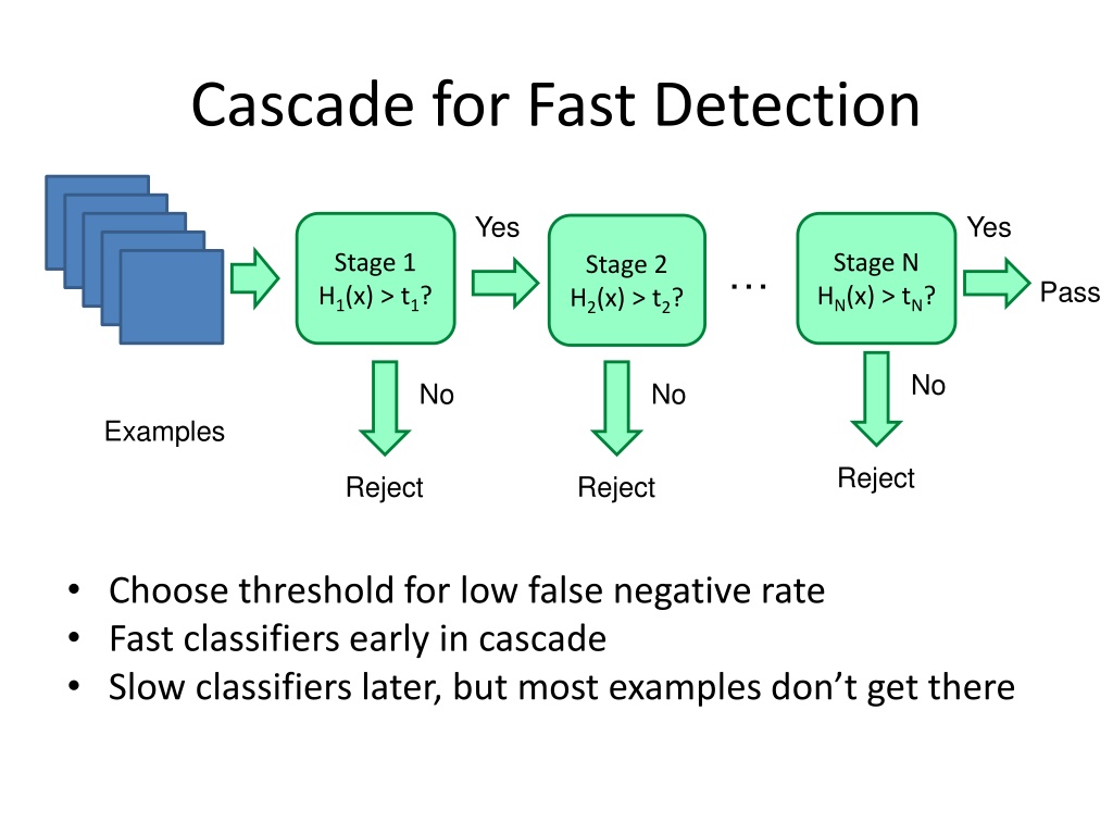
Cascade for Fast Detection
•
Choose threshold for low false negative rate
•
Fast classifiers early in cascade
•
Slow classifiers later, but most examples don’t get there
Features that are fast to compute
•
“Haar-like features”
–
Differences of sums of intensity
–
Thousands, computed at various positions and
scales within detection window
Two-rectangle features
Three-rectangle features
Etc.
-1
+1
Integral Images
•
ii = cumsum(cumsum(im, 1), 2)
x, y
ii(x,y) = Sum of the values in the grey region
SUM within Rectangle D is
ii(4) - ii(2) - ii(3) + ii(1)
Feature selection with Adaboost
•
Create a large pool of features (180K)
•
Select features that are discriminative and work
well together
–
“Weak learner” = feature + threshold + parity
–
Choose weak learner that minimizes error on the
weighted training set
–
Reweight
Adaboost
Viola-Jones details
•
38 stages with 1, 10, 25, 50 … features
–
6061 total used out of 180K candidates
–
10 features evaluated on average
•
Training Examples
–
4916 positive examples
–
10000 negative examples collected after each stage
•
Scanning
–
Scale detector rather than image
–
Scale steps = 1.25 (factor between two consecutive scales)
–
Translation 1*scale (# pixels between two consecutive windows)
•
Non-max suppression: average coordinates of overlapping
boxes
•
Train 3 classifiers and take vote
Viola Jones Results
MIT + CMU face dataset
Speed = 15 FPS (in 2001)
Object Detection
•
Overview
•
Viola-Jones
•
Dalal-Triggs
•
Deformable models
•
Deep learning
Statistical Template
Object model = sum of scores of features at fixed
positions
+
3
+
2
-
2
-
1
-
2
.
5
=
-
0
.
5
+
4
+
1
+
0
.
5
+
3
+
0
.
5
=
1
0
.
5
>
7
.
5
?
>
7
.
5
?
N
o
n
-
o
b
j
e
c
t
O
b
j
e
c
t
Design challenges
How to efficiently search for likely objects
•
Even simple models require searching hundreds of
thousands of positions and scales
Feature design and scoring
•
How should appearance be modeled? What features
correspond to the object?
How to deal with different viewpoints?
•
Often train different models for a few different
viewpoints
Implementation details
•
Window size
•
Aspect ratio
•
Translation/scale step size
•
Non-maxima suppression
Example: Dalal-Triggs pedestrian detector
1.
Extract fixed-sized (64x128 pixel) window at
each position and scale
2.
Compute HOG (histogram of gradient)
features within each window
3.
Score the window with a linear SVM classifier
4.
Perform non-maxima suppression to remove
overlapping detections with lower scores
Navneet Dalal and Bill Triggs, Histograms of Oriented Gradients for Human Detection, CVPR05
Slides by Pete Barnum
Navneet Dalal and Bill Triggs, Histograms of Oriented Gradients for Human Detection, CVPR05
•
Tested with
–
RGB
–
LAB
–
Grayscale
•
Gamma Normalization and Compression
–
Square root
–
Log
Slightly better performance vs. grayscale
Very slightly better performance vs. no adjustment
uncentered
centered
cubic-corrected
diagonal
Sobel
Slides by Pete Barnum
Navneet Dalal and Bill Triggs, Histograms of Oriented Gradients for Human Detection, CVPR05
Outperforms
•
Histogram of gradient
orientations
–
Votes weighted by magnitude
–
Bilinear interpolation between
cells
Orientation: 9 bins
(for unsigned angles
0 -180)
Histograms in
k x k pixel cells
Slides by Pete Barnum
Navneet Dalal and Bill Triggs, Histograms of Oriented Gradients for Human Detection, CVPR05
Normalize with respect to
surrounding cells
Slides by Pete Barnum
Navneet Dalal and Bill Triggs, Histograms of Oriented Gradients for Human Detection, CVPR05
X=
Slides by Pete Barnum
Navneet Dalal and Bill Triggs, Histograms of Oriented Gradients for Human Detection, CVPR05
# features = 15 x 7 x 9 x 4 = 3780
# cells
# orientations
# normalizations by
neighboring cells
Original Formulation
X=
Slides by Pete Barnum
Navneet Dalal and Bill Triggs, Histograms of Oriented Gradients for Human Detection, CVPR05
# features = 15 x 7 x 9 x 4 = 3780
# cells
# orientations
# normalizations by
neighboring cells
# features = 15 x 7 x (3 x 9) + 4 = 3780
# cells
# orientations
magnitude of
neighbor cells
UoCTTI variant
Original Formulation
Slides by Pete Barnum
Navneet Dalal and Bill Triggs, Histograms of Oriented Gradients for Human Detection, CVPR05
pos w
neg w
pedestrian
Slides by Pete Barnum
Navneet Dalal and Bill Triggs, Histograms of Oriented Gradients for Human Detection, CVPR05
Pedestrian detection with HOG
•
Train a pedestrian template using a linear support vector
machine
•
At test time, convolve feature map with template
•
Find local maxima of response
•
For multi-scale detection, repeat over multiple levels of a HOG
pyramid
N. Dalal and B. Triggs,
Histograms of Oriented Gradients for Human Detection
,
CVPR 2005
Template
HOG feature map
Detector response map
Something to think about…
•
Sliding window detectors work
–
very well
for faces
–
fairly well
for cars and pedestrians
–
badly
for cats and dogs
•
Why are some classes easier than others?
Strengths and Weaknesses of Statistical Template
Approach
Strengths
•
Works very well for non-deformable objects with
canonical orientations: faces, cars, pedestrians
•
Fast detection
Weaknesses
•
Not so well for highly deformable objects or “stuff”
•
Not robust to occlusion
•
Requires lots of training data
Tricks of the trade
•
Details in feature computation really matter
–
E.g., normalization in Dalal-Triggs improves detection rate
by 27% at fixed false positive rate
•
Template size
–
Typical choice is size of smallest detectable object
•
“Jittering” to create synthetic positive examples
–
Create slightly rotated, translated, scaled, mirrored
versions as extra positive examples
•
Bootstrapping to get hard negative examples
1.
Randomly sample negative examples
2.
Train detector
3.
Sample negative examples that score > -1
4.
Repeat until all high-scoring negative examples fit in
memory
Things to remember
•
Sliding window for search
•
Features based on differences of
intensity (gradient, wavelet, etc.)
–
Excellent results require careful feature
design
•
Boosting for feature selection
•
Integral images, cascade for speed
•
Bootstrapping to deal with many,
many negative examples
Object detection techniques employ cascades, Haar-like features, integral images, feature selection with Adaboost, and statistical modeling for efficient and accurate detection. The Viola-Jones algorithm, Dalal-Triggs method, deformable models, and deep learning approaches are prominent in this field, producing remarkable outcomes such as 15 FPS speed in face detection. The example of the Dalal-Triggs pedestrian detector showcases the process of window extraction, HOG feature computation, scoring with SVM classifier, and non-maxima suppression. References to significant works in object detection such as the Viola-Jones algorithm and Dalal-Triggs method are included.

Download Presentation

Please find below an Image/Link to download the presentation.
The content on the website is provided AS IS for your information and personal use only. It may not be sold, licensed, or shared on other websites without obtaining consent from the author.If you encounter any issues during the download, it is possible that the publisher has removed the file from their server.
You are allowed to download the files provided on this website for personal or commercial use, subject to the condition that they are used lawfully. All files are the property of their respective owners.
The content on the website is provided AS IS for your information and personal use only. It may not be sold, licensed, or shared on other websites without obtaining consent from the author.
E N D
Presentation Transcript
Cascade for Fast Detection Yes Yes Stage 1 H1(x) > t1? Stage N HN(x) > tN? Stage 2 H2(x) > t2? Pass No No No Examples Reject Reject Reject Choose threshold for low false negative rate Fast classifiers early in cascade Slow classifiers later, but most examples don t get there
Features that are fast to compute Haar-like features Differences of sums of intensity Thousands, computed at various positions and scales within detection window -1 +1 Two-rectangle features Three-rectangle features Etc.
Integral Images ii = cumsum(cumsum(im, 1), 2) x, y ii(x,y) = Sum of the values in the grey region SUM within Rectangle D is ii(4) - ii(2) - ii(3) + ii(1)
Feature selection with Adaboost Create a large pool of features (180K) Select features that are discriminative and work well together Weak learner = feature + threshold + parity Choose weak learner that minimizes error on the weighted training set Reweight
Viola Jones Results Speed = 15 FPS (in 2001) MIT + CMU face dataset
Object Detection Overview Viola-Jones Dalal-Triggs Deformable models Deep learning
Statistical Template Object model = sum of scores of features at fixed positions ? +3+2 -2-1 -2.5 = -0.5 > 7.5 Non-object ? +4+1+0.5+3+0.5= 10.5 > 7.5 Object
Example: Dalal-Triggs pedestrian detector 1. Extract fixed-sized (64x128 pixel) window at each position and scale 2. Compute HOG (histogram of gradient) features within each window 3. Score the window with a linear SVM classifier 4. Perform non-maxima suppression to remove overlapping detections with lower scores Navneet Dalal and Bill Triggs, Histograms of Oriented Gradients for Human Detection, CVPR05
Navneet Dalal and Bill Triggs, Histograms of Oriented Gradients for Human Detection, CVPR05 Slides by Pete Barnum
Tested with RGB LAB Grayscale Gamma Normalization and Compression Square root Log Slightly better performance vs. grayscale Very slightly better performance vs. no adjustment
Outperforms centered diagonal uncentered cubic-corrected Sobel Navneet Dalal and Bill Triggs, Histograms of Oriented Gradients for Human Detection, CVPR05 Slides by Pete Barnum
Histogram of gradient orientations Orientation: 9 bins (for unsigned angles 0 -180) Histograms in k x k pixel cells Votes weighted by magnitude Bilinear interpolation between cells Navneet Dalal and Bill Triggs, Histograms of Oriented Gradients for Human Detection, CVPR05 Slides by Pete Barnum
Normalize with respect to surrounding cells Navneet Dalal and Bill Triggs, Histograms of Oriented Gradients for Human Detection, CVPR05 Slides by Pete Barnum
Original Formulation # orientations # features = 15 x 7 x 9 x 4 = 3780 X= # cells # normalizations by neighboring cells Navneet Dalal and Bill Triggs, Histograms of Oriented Gradients for Human Detection, CVPR05 Slides by Pete Barnum
neg w pos w Navneet Dalal and Bill Triggs, Histograms of Oriented Gradients for Human Detection, CVPR05 Slides by Pete Barnum
pedestrian Navneet Dalal and Bill Triggs, Histograms of Oriented Gradients for Human Detection, CVPR05 Slides by Pete Barnum
Pedestrian detection with HOG Train a pedestrian template using a linear support vector machine At test time, convolve feature map with template Find local maxima of response For multi-scale detection, repeat over multiple levels of a HOG pyramid HOG feature map Detector response map Template N. Dalal and B. Triggs, Histograms of Oriented Gradients for Human Detection, CVPR 2005
Something to think about Sliding window detectors work very well for faces fairly well for cars and pedestrians badly for cats and dogs Why are some classes easier than others?
Strengths and Weaknesses of Statistical Template Approach Strengths Works very well for non-deformable objects with canonical orientations: faces, cars, pedestrians Fast detection Weaknesses Not so well for highly deformable objects or stuff Not robust to occlusion Requires lots of training data
Tricks of the trade Details in feature computation really matter E.g., normalization in Dalal-Triggs improves detection rate by 27% at fixed false positive rate Template size Typical choice is size of smallest detectable object Jittering to create synthetic positive examples Create slightly rotated, translated, scaled, mirrored versions as extra positive examples Bootstrapping to get hard negative examples 1. Randomly sample negative examples 2. Train detector 3. Sample negative examples that score > -1 4. Repeat until all high-scoring negative examples fit in memory
Things to remember Sliding window for search Features based on differences of intensity (gradient, wavelet, etc.) Excellent results require careful feature design Boosting for feature selection Integral images, cascade for speed Yes Yes Stage 1 H1(x) > t1? Stage N HN(x) > tN? Stage 2 H2(x) > t2? Pass No Bootstrapping to deal with many, many negative examples No No Examples Reject Reject Reject