NUTS AND BOLTS OF DFT CALCULATIONS

NUTS AND BOLTS OF DFT

NUTS AND BOLTS OF DFT

CALCULATIONS

CALCULATIONS

3.1 RECIPROCAL SPACE AND k POINTS

3.1 RECIPROCAL SPACE AND k POINTS

3.1.1 Plane Waves and the Brillouin Zone

3.1.1 Plane Waves and the Brillouin Zone

If we solve the Schrödinger equation for this periodic

If we solve the Schrödinger equation for this periodic

system, the solution must satisfy a fundamental property

system, the solution must satisfy a fundamental property

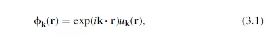
known as Bloch’s theorem, which states that the solution

known as Bloch’s theorem, which states that the solution

can be expressed as a sum of terms with the form:

can be expressed as a sum of terms with the form:

where u

where u

k

k

(r) is periodic in space with the same periodicity as

(r) is periodic in space with the same periodicity as

the supercell.

the supercell.

2

The space of vectors k is called reciprocal space (or simply k space).

The space of vectors k is called reciprocal space (or simply k space).

We define three vectors that define positions in reciprocal space.

We define three vectors that define positions in reciprocal space.

These vectors are called the reciprocal lattice vectors, b

These vectors are called the reciprocal lattice vectors, b

1

1

, b

, b

2

2

, and

, and

b

b

3

3

, and are defined so that a

, and are defined so that a

i

i

·b

·b

j

j

 is 2

 is 2

π

π

 if i=j and 0 otherwise. This

 if i=j and 0 otherwise. This

choice means that

choice means that

3

4

We can define a primitive cell in reciprocal space. Because

We can define a primitive cell in reciprocal space. Because

this cell has many special properties, it is given a name: it is

this cell has many special properties, it is given a name: it is

the Brillouin zone (often abbreviated to BZ).

the Brillouin zone (often abbreviated to BZ).

5

3.1.2 Choosing k Points in the Brillouin Zone

3.1.2 Choosing k Points in the Brillouin Zone

The solution that is used most widely was developed by

The solution that is used most widely was developed by

Monkhorst and Pack in 1976. Most DFT packages offer the

Monkhorst and Pack in 1976. Most DFT packages offer the

option of choosing k points based on this method.

option of choosing k points based on this method.

In practice, how should we choose how many k points to use?

In practice, how should we choose how many k points to use?

6

7

8

The last column in Table 3.2 lists the computational time

The last column in Table 3.2 lists the computational time

taken for the total energy calculations, normalized by the

taken for the total energy calculations, normalized by the

result for M=1.

result for M=1.

if M is an odd number, then the amount of time taken for the

if M is an odd number, then the amount of time taken for the

calculations with either M or (M+1) was close to the same.

calculations with either M or (M+1) was close to the same.

This occurs because the calculations take full advantage of the

This occurs because the calculations take full advantage of the

many 

many 

symmetries

symmetries

 that exist in a perfect fcc solid.

 that exist in a perfect fcc solid.

9

This reduced region in k space is called the 

This reduced region in k space is called the 

irreducible

irreducible

Brillouin zone (IBZ)

Brillouin zone (IBZ)

.

.

To show how helpful symmetry is in reducing the work

To show how helpful symmetry is in reducing the work

required for a DFT calculation, we have repeated some of

required for a DFT calculation, we have repeated some of

the calculations from Table 3.2 for a four-atom supercell in

the calculations from Table 3.2 for a four-atom supercell in

which each atom was given a slight displacement away

which each atom was given a slight displacement away

from its fcc lattice position.

from its fcc lattice position.

10

11

3.1.3 Metals—Special Cases in k Space

3.1.3 Metals—Special Cases in k Space

One useful definition of a metal is that in a metal the Brillouin

One useful definition of a metal is that in a metal the Brillouin

zone can be divided into regions that are occupied and

zone can be divided into regions that are occupied and

unoccupied by electrons. The surface in k space that separates

unoccupied by electrons. The surface in k space that separates

these two regions is called the 

these two regions is called the 

Fermi surface

Fermi surface

.

.

12

We will describe the two best-known methods to solve the

We will describe the two best-known methods to solve the

problem of slow convergence of metal calculations.

problem of slow convergence of metal calculations.

The first is called 

The first is called 

the tetrahedron method

the tetrahedron method

.

.

The idea behind this method is 

The idea behind this method is 

to use the discrete set of k

to use the discrete set of k

points to define a set of tetrahedra that fill reciprocal space

points to define a set of tetrahedra that fill reciprocal space

and to define the function being integrated at every point in a

and to define the function being integrated at every point in a

tetrahedron using interpolation.

tetrahedron using interpolation.

13

A different approach to the discontinuous integrals that

A different approach to the discontinuous integrals that

appear for metals are 

appear for metals are 

the smearing methods.

the smearing methods.

The idea of these methods is 

The idea of these methods is 

to force the function being

to force the function being

integrated to be continuous by “smearing” out the

integrated to be continuous by “smearing” out the

discontinuity.

discontinuity.

14

An example of a smearing function is the Fermi–Dirac

An example of a smearing function is the Fermi–Dirac

function:

function:

Figure 3.3 shows the shape of this function for several

Figure 3.3 shows the shape of this function for several

values of 

values of 

σ

σ

.

.

15

16

3.1.4 Summary of k Space

3.1.4 Summary of k Space

The key ideas related to getting well-converged results in k

The key ideas related to getting well-converged results in k

space include:

space include:

1. Before pursuing a large series of DFT calculations for a

1. Before pursuing a large series of DFT calculations for a

system of interest, numerical data exploring the

system of interest, numerical data exploring the

convergence of the calculations with respect to the number

convergence of the calculations with respect to the number

of k points should be obtained.

of k points should be obtained.

2. The number of k points used in any calculation should be

2. The number of k points used in any calculation should be

reported since not doing so makes reproduction of the

reported since not doing so makes reproduction of the

result difficult.

result difficult.

17

3. Increasing the volume of a supercell reduces the number

3. Increasing the volume of a supercell reduces the number

of k points needed to achieve convergence because volume

of k points needed to achieve convergence because volume

increases in real space correspond to volume decreases in

increases in real space correspond to volume decreases in

reciprocal space.

reciprocal space.

4. If calculations involving supercells with different volumes

4. If calculations involving supercells with different volumes

are to be compared, choosing k points so that the density

are to be compared, choosing k points so that the density

of k points in reciprocal space is comparable for the

of k points in reciprocal space is comparable for the

different supercells is a useful way to have comparable

different supercells is a useful way to have comparable

levels of convergence in k space.

levels of convergence in k space.

18

5. Understanding how symmetry is used to reduce the

5. Understanding how symmetry is used to reduce the

number of k points for which calculations are actually

number of k points for which calculations are actually

performed can help in understanding how long individual

performed can help in understanding how long individual

calculations will take. But overall convergence is

calculations will take. But overall convergence is

determined by the density of k points in the full Brillouin

determined by the density of k points in the full Brillouin

zone, not just the number of k points in the irreducible

zone, not just the number of k points in the irreducible

Brillouin zone.

Brillouin zone.

6. Appropriate methods must be used to accurately treat k

6. Appropriate methods must be used to accurately treat k

space for metals.

space for metals.

19

3.2 ENERGY CUTOFFS

3.2 ENERGY CUTOFFS

Our lengthy discussion of k space began with Bloch’s

Our lengthy discussion of k space began with Bloch’s

theorem, which tells us that solutions of the Schrödinger

theorem, which tells us that solutions of the Schrödinger

equation for a supercell have the form

equation for a supercell have the form

where u

where u

k

k

(r) is periodic in space with the same periodicity as

(r) is periodic in space with the same periodicity as

the supercell. It is now time to look at this part of the

the supercell. It is now time to look at this part of the

problem more carefully. The periodicity of u

problem more carefully. The periodicity of u

k

k

(r) means that

(r) means that

it can be expanded in terms of a special set of plane waves:

it can be expanded in terms of a special set of plane waves:

20

Combining the two equations above gives:

Combining the two equations above gives:

The functions appearing in Eq.(3.13) have a simple

The functions appearing in Eq.(3.13) have a simple

interpretation as solutions of the Schrödinger equation:

interpretation as solutions of the Schrödinger equation:

they are solutions with kinetic energy:

they are solutions with kinetic energy:

21

As a result, it is usual to truncate the infinite sum above to

As a result, it is usual to truncate the infinite sum above to

include only solutions with kinetic energies less than some

include only solutions with kinetic energies less than some

value:

value:

The infinite sum then reduces to :

The infinite sum then reduces to :

22

23

3.2.1 Pseudopotentials

3.2.1 Pseudopotentials

A pseudopotential replaces the electron density

A pseudopotential replaces the electron density

from a chosen set of core electrons with a smoothed

from a chosen set of core electrons with a smoothed

density chosen to match various important physical

density chosen to match various important physical

and mathematical properties of the true ion core.

and mathematical properties of the true ion core.

24

A pseudopotential is developed by considering an

A pseudopotential is developed by considering an

isolated atom of one element, but the resulting

isolated atom of one element, but the resulting

pseudopotential can then 

pseudopotential can then 

be used reliably for

be used reliably for

calculations that place this atom in any chemical

calculations that place this atom in any chemical

environment

environment

without further adjustment

without further adjustment

 of the

 of the

pseudopotential.

pseudopotential.

25

3.3 NUMERICAL OPTIMIZATION

3.3 NUMERICAL OPTIMIZATION

To make practical use of our ability to perform numerically

To make practical use of our ability to perform numerically

converged DFT calculations, we also need methods that can

converged DFT calculations, we also need methods that can

help us effectively cope with situations where we want to

help us effectively cope with situations where we want to

search through a problem with many degrees of freedom.

search through a problem with many degrees of freedom.

26

3.3.1 Optimization in One Dimension

3.3.1 Optimization in One Dimension

How to find a local minimum of f (x)?

How to find a local minimum of f (x)?

The first approach is the 

The first approach is the 

bisection method

bisection method

.

.

The second approach is 

The second approach is 

Newton’s method

Newton’s method

.

.

27

28

A striking difference between the bisection method and

A striking difference between the bisection method and

Newton’s method is how rapidly the solutions converge.

Newton’s method is how rapidly the solutions converge.

29

Newton’s method is better than the bisection method

Newton’s method is better than the bisection method

How do we know when to stop?

How do we know when to stop?

A typical choice is to continue iterating until the

A typical choice is to continue iterating until the

difference between successive iterates is smaller

difference between successive iterates is smaller

than some tolerance:

than some tolerance:

30

there are several general properties of numerical

there are several general properties of numerical

optimization that are extremely important to appreciate.

optimization that are extremely important to appreciate.

They include :

They include :

1. The algorithms are iterative, so they do not provide an

1. The algorithms are iterative, so they do not provide an

exact solution; instead, they provide a series of

exact solution; instead, they provide a series of

approximations to the exact solution.

approximations to the exact solution.

2. An initial estimate for the solution must be provided to

2. An initial estimate for the solution must be provided to

use the algorithms.The algorithms provide no guidance on

use the algorithms.The algorithms provide no guidance on

how to choose this initial estimate.

how to choose this initial estimate.

31

3. The number of iterations performed is controlled by a

3. The number of iterations performed is controlled by a

tolerance parameter that estimates how close the current

tolerance parameter that estimates how close the current

solution is to the exact solution.

solution is to the exact solution.

4. Repeating any algorithm with a different tolerance

4. Repeating any algorithm with a different tolerance

parameter or a different initial estimate for the solution will

parameter or a different initial estimate for the solution will

generate multiple final approximate solutions that are

generate multiple final approximate solutions that are

(typically) similar but are not identical.

(typically) similar but are not identical.

5. The rate at which different algorithms converge to a

5. The rate at which different algorithms converge to a

solution can vary greatly, so choosing an appropriate

solution can vary greatly, so choosing an appropriate

algorithm can greatly reduce the number of iterations

algorithm can greatly reduce the number of iterations

needed.

needed.

32

6. These methods cannot tell us if there are multiple minima

6. These methods cannot tell us if there are multiple minima

of the function we are considering if we just apply the

of the function we are considering if we just apply the

method once. Applying a method multiple times with

method once. Applying a method multiple times with

different initial estimates can yield multiple minima, but

different initial estimates can yield multiple minima, but

even in this case the methods do not give enough

even in this case the methods do not give enough

information to prove that all possible minima have been

information to prove that all possible minima have been

found.

found.

7. For most methods, no guarantees can be given that the

7. For most methods, no guarantees can be given that the

method will converge to a solution at all for an arbitrary

method will converge to a solution at all for an arbitrary

initial estimate.

initial estimate.

33

3.3.2 Optimization in More than One Dimension

3.3.2 Optimization in More than One Dimension

The one-dimensional Newton method was derived using a

The one-dimensional Newton method was derived using a

Taylor expansion, and the multidimensional problem can be

Taylor expansion, and the multidimensional problem can be

approached in the same way.

approached in the same way.

Newton’s method defines a series of iterates by:

Newton’s method defines a series of iterates by:

34

Unfortunately, Newton’s method simply cannot be

Unfortunately, Newton’s method simply cannot be

applied to the DFT problem we set ourselves at the

applied to the DFT problem we set ourselves at the

beginning of this section!

beginning of this section!

35

It is very difficult to directly evaluate second

It is very difficult to directly evaluate second

derivatives of energy within plane-wave DFT, and

derivatives of energy within plane-wave DFT, and

most codes do not attempt to perform these

most codes do not attempt to perform these

calculations.

calculations.

36

As a result, we have to look for other approaches to

As a result, we have to look for other approaches to

minimize E(x). We will briefly discuss the two

minimize E(x). We will briefly discuss the two

numerical methods that are most commonly used

numerical methods that are most commonly used

for this problem: 

for this problem: 

quasi-Newton

quasi-Newton

 and 

 and 

conjugate-

conjugate-

gradient methods

gradient methods

.

.

37

The essence of 

The essence of 

quasi-Newton methods

quasi-Newton methods

 is to replace Eq.

 is to replace Eq.

(3.15) by :

(3.15) by :

where A

where A

i

i

 is a matrix that is defined to approximate the

 is a matrix that is defined to approximate the

Jacobian matrix. This matrix is also updated iteratively

Jacobian matrix. This matrix is also updated iteratively

during the calculation and has the form:

during the calculation and has the form:

38

Conjugate gradient method:

Conjugate gradient method:

We begin with an initial estimate, x

We begin with an initial estimate, x

0

0

. Our first iterate is

. Our first iterate is

chosen to lie along the direction defined by

chosen to lie along the direction defined by

the problem of choosing the best value of 

the problem of choosing the best value of 

α

α

0

0

 cannot be

 cannot be

solved exactly. Choose the step size by some approximate

solved exactly. Choose the step size by some approximate

method that may be as simple as evaluating E

method that may be as simple as evaluating E

(x1) 

(x1) 

for several

for several

possible step lengths and selecting the best result.

possible step lengths and selecting the best result.

39

3

3

.

.

4

4

G

G

E

E

O

O

M

M

E

E

T

T

R

R

Y

Y

O

O

P

P

T

T

I

I

M

M

I

I

Z

Z

A

A

T

T

I

I

O

O

N

N

3.4.1 Internal Degrees of Freedom

3.4.1 Internal Degrees of Freedom

Example 1 : Obtain the energy of the gas phase N

Example 1 : Obtain the energy of the gas phase N

2 

2 

molecule

molecule

Step 1 :Create a cubic super-cell with a side length of L

Step 1 :Create a cubic super-cell with a side length of L

Step 2 :Place two N atoms at the fractional coordinates (0,

Step 2 :Place two N atoms at the fractional coordinates (0,

0, 0) and ( + d/L , O , 0) of this supercell.

0, 0) and ( + d/L , O , 0) of this supercell.

Step 3:find the DFT-optimized bond length for N

Step 3:find the DFT-optimized bond length for N

2

2

 by using

 by using

either the quasi-Newton or conjugate-gradient methods

either the quasi-Newton or conjugate-gradient methods

defined above to minimize the total energy of our supercell.

defined above to minimize the total energy of our supercell.

40

Example 2 : Optimize the geometry of a molecule of CO

Example 2 : Optimize the geometry of a molecule of CO

2

2

Step 1 :Create a cubic super-cell with a side length of L

Step 1 :Create a cubic super-cell with a side length of L

Step 2 :Create a CO2 molecule by placing a C atom at

Step 2 :Create a CO2 molecule by placing a C atom at

fractional coordinates (0,0,0) and O atoms at (+d/L,0,0) and

fractional coordinates (0,0,0) and O atoms at (+d/L,0,0) and

(-d/L,0,0).

(-d/L,0,0).

Step 3:find the DFT-optimized bond length for CO

Step 3:find the DFT-optimized bond length for CO

2

2

 by using

 by using

either the quasi-Newton or conjugate-gradient methods

either the quasi-Newton or conjugate-gradient methods

defined above to minimize the total energy of our supercell.

defined above to minimize the total energy of our supercell.

41

3.4.2 Geometry Optimization with Constrained

3.4.2 Geometry Optimization with Constrained

Atoms

Atoms

There are many types of calculations where it is useful to

There are many types of calculations where it is useful to

minimize the energy of a supercell by optimizing the

minimize the energy of a supercell by optimizing the

position of some atoms while holding other atoms at fixed

position of some atoms while holding other atoms at fixed

positions.

positions.

42