Maximization Problems with Submodular Objective Functions


Maximization Problems with
Submodular Objective Functions
Moran Feldman
Publication List
•
Improved Approximations for k-Exchange Systems.
Moran Feldman, Joseph (Seffi) Naor, Roy Schwartz and Justin Ward, ESA, 2011.
•
A Unified Continuous Greedy Algorithm for Submodular Maximization.
Moran Feldman, Joseph (Seffi) Naor and Roy Schwartz, FOCS 2011.
•
A Tight Linear Time (1/2)-Approximation for Unconstrained Submodular Maximization.
Niv Buchbinder, Moran Feldman, Joseph (Seffi) Naor and Roy Schwartz, FOCS 2012.


Outline
•
Preliminaries
–
What is a submodular function?
•
Unconstrained Submodular Maximization
•
More Preliminaries
•
Maximizining a Submodular Function over a
Polytope Constraint
2

Set Functions
Definition
Given a ground set
N
, a set function
f
: 2
N
R
assigns a number to
every subset of the ground set.
Intuition
•
Consider a player participating in an auction on a set
N
of
elements.
•
The utility of the player from buying a subset
N
’
N
of elements
is given by a set function
f
.
Modular Functions
A set function is modular (linear) if there is a fixed utility
v
u
for every
element
u
N
, and the utility of a subset
N’
N
is given by:
3
Properties of Set Functions
Motivation
•
Modularity is often a too strong property.
•
Many weaker properties have been defined.
•
A modular function has all these properties.
4
Properties of Set Functions (cont.)
Difficulty
•
Subadditivity is often a too weak property.
Solution
•
A stronger property called submodularity.
•
The marginal contribution of an element
u
to a set
A
decreases
when adding elements to
A.
Notation
Given a set
A
, and an elements
u
,
f
u
(
A
) is the marginal contribution of
u
to
A
:
Formal Definition
5
For sets
A
B
N
, and
u
B
:
f
u
(
A
)
f
u
(
B
)
For sets
A
,
B
N
:
f
(
A
) +
f
(
B
)
f
(
A
B
) +
f
(
A
B
)
Submodular Function - Example
6
0
5
6
7
10
8
11
0
Too
heavy
•
Normalized
•
Nonmonotone
•
Submodular
5
4
-8
Where can One Find Submodular Set Functions?
Question
Submodularity looks peculiar. Is it common in real life?
Answer
•
Yes, submodular set functions pop often in many settings.
•
Submodular functions represents “economy of scale”, which
makes them useful in economics.
•
Examples of submodular functions in combinatorial settings:
7
Unconstrained Submodular Maximization
Instance
A non-negative submodular function
f
: 2
N
R
+
.
Objective
Find a subset
S
N
maximizing
f
(
S
).
Most Recent Previous Works
•
0.41 approximation via simulated annealing [Gharan and
Vondrak 11]
•
0.42 approximation via a combination of simulated
annealing and the Structural Continuous Greedy Algorithm
[Feldman et al. 11]
•
0.5 hardness [Feige et al. 07]
8
The Players
•
The algorithm we present manages two solutions (sets):
–
X
– Initially the empty set.
–
Y – Initially the set of all elements (
N
).
•
The elements are ordered in an arbitrary order:
u
1
,
u
2
, …,
u
n
.
•
The algorithm has
n
iterations, one for each element. In iteration
i
the algorithm decides whether to add
u
i
to
X
or to remove it from
Y
.
•
The following notation is defined using these players:
9
Formally:
The contribution
of adding
u
i
to
X
a
i
=
f
(
X
{u
i
}) –
f
(
X
)
The contribution of
removing
u
i
from
Y
b
i
=
f
(
Y
\ {u
i
}) –
f
(
Y
)
More on the Algorithm
•
Above we can see the initial configuration of the algorithm.
–
The set
Y
is red. Initially it contains all the elements.
–
The set
X
is green. Initially it contains no elements.
•
Assume the algorithm now performs the following moves:
–
Add
u
1
to
X
.
–
Remove
u
2
from
Y
.
–
Add
u
3
to
X
.
–
Add
u
4
to
X
.
–
Remove
u
5
from
Y
.
•
Notice: when the algorithm terminates,
X
=
Y
is the output
of the algorithm.
10
Notation
•
X
i
and
Y
i
- the values of the sets
X
and
Y
after
i
iterations.
•
OPT
i
- the optimal set such that:
X
i
OPT
i
Y
i
.
•
V
– the value of the algorithm’s output.
11
For
i
= 0
OPT
0
= OPT
X
0
=
Y
0
=
N
For
i
=
n
OPT
n
=
X
n
=
Y
n
f
(
OPT
n
) =
f
(
X
n
) =
f
(
Y
n
) =
V
Observations
•
As
i
increases,
f
(
OPT
i
) deteriorates from
f
(
OPT
) to
V
.
•
V
[
f
(
X
n
) –
f
(
X
0
) +
f
(
Y
n
) –
f
(
Y
0
)] / 2,
i.e.
,
V
is at least the increase in
f
(
X
) +
f
(
Y
) over 2.
Roadmap
•
To analyze the algorithm we show that for some constant
c
and every iteration
i
:
12
•
Summing over all the iterations, we get:
Deterioration in OPT
c ∙
Improvement in
f
(
X
) +
f
(
Y
)
f
(
OPT
) -
V
2
c ∙
V
V
f
(
OPT
) / [1 + 2
c
]
•
The value of
c
depends on how the algorithm decides
whether to add
u
i
to
X
or remove it from
Y
.
(*)
Deterministic Rule
If
a
i
b
i
•
then
add
u
i
to
X
,
•
else remove
u
i
from
Y
.
Lemma
Always,
a
i
+
b
i
0
.
Lemma
If the algorithm adds
u
i
to X
(respectively, removes
u
i
from
Y
),
and
OPT
i-1
OPT
i
, then
the deterioration in
OPT
is at most
b
i
(respectively,
a
i
).
Proof
Since
OPT
i-1
OPT
i
,
we know that
u
i
OPT
i
-1
.
13
Non-standard
greedy algorithm
f
(
OPT
i
-1
) –
f
(
OPT
i
)
f
(
OPT
i
-1
) –
f
(
OPT
i-1
{u
i
}
)
f
(
Y
\ {u
i
}) –
f
(
Y
) =
b
i
Deterministic Rule - Analysis
•
Assume
a
i
b
i
, and the algorithm
adds
u
i
to
X
(the other case is analogues
).
•
Cleary
a
i
0 since
a
i
+
b
i
0.
•
If
u
i
OPT
i
-1
, then:
–
f
(
OPT
i-1
) -
f
(
OPT
i
) = 0
–
f
(
X
i
) –
f
(
X
i
-1
) +
f
(
Y
i
) –
f
(
Y
i
-1
) =
a
i
0
–
Inequality (*) holds for every non-negative
c
.
•
If
u
i
OPT
i
-1
, then:
–
f
(
OPT
i-1
) -
f
(
OPT
i
)
b
i
–
f
(
X
i
) –
f
(
X
i
-1
) +
f
(
Y
i
) –
f
(
Y
i
-1
) =
a
i
b
i
–
Inequality (*) holds for
c
= 1.
•
The approximation ratio is: 1 /
[1 + 2
c
] = 1/3.
14
Random Rule
1.
If
b
i
0, then add
u
i
to
X
and quit.
2.
If
a
i
0, then remove
u
i
from
Y
and quit.
3.
With probability
a
i
/ (
a
i
+
b
i
) add
u
i
to
X
, otherwise (with
probability
b
i
/ (
a
i
+
b
i
)), remove
u
i
from
Y
.
Three cases: one for each line of the algorithm.
Case 1 (
b
i
0)
•
Cleary
a
i
0 since
a
i
+
b
i
0.
•
Thus,
f
(
X
i
) –
f
(
X
i
-1
) +
f
(
Y
i
) –
f
(
Y
i
-1
) =
a
i
0.
•
If
u
i
OPT
i
-1
, then
f
(
OPT
i-1
) -
f
(
OPT
i
) = 0
•
If
u
i
OPT
i
-1
, then
f
(
OPT
i-1
) -
f
(
OPT
i
)
b
i
0
•
Inequality (*) holds for every non-negative
c
.
15
Random Rule - Analysis
Case 2 (
a
i
0)
Analogues to the previous case.
Case 3 (
a
i
,
b
i
> 0)
The improvement is:
Assume, w.l.o.g.,
u
i
OPT
i
-1
, t
he deterioration in OPT is:
Inequality (*) holds for
c
= 0.5, since:
The approximation ratio is: 1 /
[1 + 2
c
] = 1/2.
16
17
Polytope Constraints
•
We abuse notation and identify a set
S
with its
characteristic vector in [0, 1]
N
.
–
Given a set
S
, we use
S
also to denote its characteristic
vector.
–
Given a vector
x
{0, 1}N
, we denote by
x
also the set
whose characteristic vector is
x
.
18
•
Using this notation,
we can define LP like
problems:
•
More generally, maximizing a
submodular functrion subject
to a polytope
P
constraint is
the problem:
Relaxation
•
The last program:
–
requires integer solutions.
–
generalizes “integer programming”.
–
is unlikely to have a reasonable approximation.
•
We need to relax it.
–
We replace the constraint
x
{0,1}N
with x
[0,1]
N
.
–
The difficulty is to extend the objective function to fractional
vectors.
•
The multilinear extension
F
(a.k.a. extension by expectation)
[Calinescu et al. 07].
–
Given a vector
x
[0, 1]
N
,
let
R
(
x
) denote a random set
containing every element
u
N
with probability
x
u
independently.
–
F
(
x
)
= E[
f
(
R
(
x
))].
19
Introducing the Problem
Maximizining a Submodular Function over a Polytope Constraint
•
Asks to find (or approximate) the optimal solution for a relaxation
of the form presented.
•
Formally for as large a constant
c
as possible:
–
Given , find a feasible
x
such that:
F
(
x
)
c ∙
f
(
OPT
).
Motivation
•
For many polytopes, a fractional solution can be rounded without
losing too much in the objective.
–
Matroid Polytopes – no loss
[Calinescu et al. 11].
–
Constant number of knapsacks – (1 –
ε
) loss [Kulik et al. 09].
–
Unsplittable flow in trees – O(1) loss [
Chekuri et al. 11].
20
The Continuous Greedy Algorithm
The Algorithm [Vondrak 08]
•
Let
δ
> 0 be a small number.
1.
Initialize:
y
(0)
and
t
0.
2.
While
t
< 1 do:
3.
For every
u
N
, let
w
u
=
F
(
y
(
t
)
u
) –
F
(
y
(
t
)).
4.
Find a solution
x
in
P
[0, 1]
N
maximizing
w
∙
x
.
5.
y
(
t
+
δ
)
y
(
t
) +
δ
∙
x
6.
Set
t
t
+
δ
7.
Return
y
(
t
)
Remark
•
Calculation of
w
u
can be tricky for some functions.
•
Assuming one can evaluate
f
, the value of
w
u
can be approximated
via sampling.
21
22
The Continuous Greedy Algorithm - Demonstration
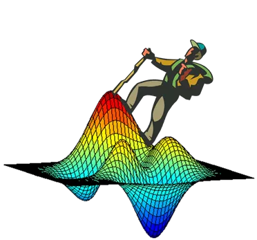
Observations
•
The algorithm is somewhat like gradient descent.
•
The algorithm moves only in positive directions because the
extension
F
is guaranteed to be concave in such directions.
y
(0)
y
(0.01)
y
(0.02)
y
(0.03)
y
(0.04)
The Continuous Greedy Algorithm - Results
Theorem
[Calinescu et al. 11]
•
Assuming,
–
f
is a normalized monotone submodular function.
–
P
is a solvable polytope.
•
The continuous greedy algorithm gives 1 – 1/
e – o
(
n
-1
)
approximation.
•
By guessing the element of
OPT
with the maximal marginal
contribution, one can get an optimal 1 – 1/
e
approximation.
Proof Idea
•
Show that
w ∙ x
w
∙
OPT
is large.
•
Show that the improvement in each iteration
δ
∙
w
∙
x
.
•
Sum up the improvements over all the iterations.
23
The Continuous Greedy Algorithm - Rethinking
Question
What is the difference between gradient descent and the
continuous greedy?
Answer
•
In gradient descent the direction chosen is the direction
x
maximizing
x
∙
F
.
•
In the continuous greedy the direction chosen is the
direction
x
maximizing
x
∙
w
, where
w
u
is the marginal
contribution of
u
.
24
The Measured Continuous Greedy Algorithm
Idea
To guarantee a gain of
δ
∙
w
∙
x
, it is enough to increase
y
u
by:
δ
∙
x
u
∙
(1 –
y
u
(
t
)).
The Algorithm
•
Let
δ
> 0 be a small number.
1.
Initialize:
y
(0)
and
t
0.
2.
While
t
<
T
do:
3.
For every
u
N
, let
w
u
=
F
(
y
(
t
)
u) –
F
(
y
(
t
)).
4.
Find a solution
x
in
P
{0, 1}N
maximizing
w
∙
x
.
5.
For every
u
N
,
y
u
(
t
+
δ
)
y
u
(
t
) +
δ
∙
x
u
∙ (1 –
y
u
(
t
))
.
6.
Set
t
t
+
δ
7.
Return
y
(
t
)
25
The Measured Continuous Greedy Algorithm - Results
Theorem
•
Assuming,
–
f
is a non-negative submodular function.
–
P
is a solvable down-montone polytope.
•
The approximation ratio of the measured continuous
greedy algorithm with
T
= 1
is 1/
e – o
(
n
-1
).
Remarks
•
For monotone
f
, we get the an approximation ratio of
1-
e
-
T
. For
T
= 1, this is the ratio of the continuous greedy.
•
The solution is no longer a convex combination of points
of
P
:
–
The sum of the coefficients is at most
T
.
–
For
T
1, the output is in
P
since
P
is down-monotone.
26
The Measured Continuous Greedy Algorithm - Analysis
Helper Lemma
Given
x
[0, 1]
N
and
[0, 1], let
T
(
x
) be a set containing every
element
u
N
such that
x
u
.
•
For every
x
[0, 1]
N
,
Proof
Omitted due to time constraints.
Lemma 1
There is a good direction,
i.e.
,
w
∙
x
e
-
t
∙
f
(
OPT
) –
F
(
y
(
t
))
.
Proof
•
Notice that the increase in
y
u
(
t
) is at most
δ
∙
(1 –
y
u
(
t
)).
•
If
δ
is infinitely small,
y
u
(
t
) is upper bounded by the solution of the
following differential equation.
•
For small
δ
,
y
u
(
t
) is
almost
upper bounded by 1 –
e
-t
.
27
The Continuous Greedy Algorithm – Analysis (cont.)
•
OPT itself is a feasible direction. Its weight is:
Lemma 2
The improvement is related to
w
∙
x
,
i.e.
,
F
(
y
(
t
+
δ
))
F
(
y
(
t
)) +
δ
∙
w
∙
x
.
Proof
•
For small
δ
:
28
Proof of the Theorem
•
Combining the last two lemmata gives:
F
(
y
(
t
+
δ
)) -
F
(
y
(
t
))
δ
∙
[
e
-
t
∙
f
(
OPT
) –
F
(
y
(
t
))]
•
Let
g
(
t
) =
F
(
y
(
t
)). For small
δ
the last equation becomes
the differential equation:
dg
/
dt
=
e
-
t
∙
f
(
OPT
) –
g
(
t
),
g
(0) = 0
•
The solution of this equation is:
g
(
t
) =
t
∙
e
-
t
∙
f
(OPT)
•
Hence, at time
t
= 1, the value of the solution is at least
g
(1) =
e
-1
∙
f
(OPT)
.
29
Result for Monotone Functions
•
For non-monotone functions, the approximation
ratio is
T
∙
e
-T
, which is maximized for
T
= 1.
•
For monotone functions, the approximation ratio
is 1 –
e
-
T
, which improves as
T
increases.
•
In general, the solution produced for
T
> 1:
–
Is always within the cube [0, 1]
N
.
–
Might be outside the polytope.
•
However, for some polytopes, somewhat larger
values of
T
can be used.
30
31
The Submodular Welfare Problem
Instance
•
A set
P
of
n
players
•
A set
Q
of
m
items
•
Normalized monotone submodular utility function
w
j
: 2
Q
R
+
for each player.
Objective
•
Let
Q
j
Q
denote the set of items the
j
th
player gets.
•
The utility of the
j
th
player is
w
j
(
Q
j
).
•
Distribute the items among the players, maximizing the sum
of utilities.
The Polytope
Problem Representation
•
Each item is represented by
n
elements in the ground set (each one
corresponding to its assignment to a different player).
•
The objective is the sum of the utility functions of the players, each
applied to the items allocated to it.
•
The polytope requires that every item will be allocated to at most
one player.
Analyzing a Single Constraint
•
All constraints are of the form:
•
Let
t
i
be the amount of time in which the algorithm increases
x
i
.
Notice that
x
i
= 1 –
e
-t
i
.
•
By definition, , and it can be shown that for
T
-
n
∙ ln (1–n
-1
)
it always holds that:
32
Approximating the Submodular Welfare Problem
•
Apply the measured continuous greedy till time:
T
= -
n
∙ ln (1 – 1/n)
•
By the previous analysis, the solution produced
will be in the polytope.
•
The expected value of the solution is at least:
•
Round the solution using the natural rounding:
–
Assign an item to each player with probability equal to
the corresponding variable.
•
This approximation ratio is tight for every
n
.
[Vondrak 06]
33
Open Problems
•
The measured continuous greedy algorithm:
–
Provides tight approximation for monotone functions
[Nemhauser and Wolsey 78].
–
Is this also the case for non-monotone functions?
–
The current approximation ratio of
e
-1
is a natural
number.
•
Uniform Matroids
–
The approximability depends on
k
/
n
.
•
For
k
/
n
= 0.5, we have 0.5 approximation.
•
Recently, a hardness of a bit less than 0.5 was shown for
k/n
approaching 0
.
[Gharan and Vondrak 11]
–
What is the correct approximation ratio as a function
of
k
/
n
?
–
We know it is always possible to bit the
e
-1
ratio.
34
In the study of submodular set functions, this publication delves into the properties, examples, and applications of such functions in various domains like economics and combinatorial settings. Submodular functions exhibit characteristics such as modularity, normalization, and monotonicity, making them valuable for optimization problems and resource allocation.

Download Presentation

Please find below an Image/Link to download the presentation.
The content on the website is provided AS IS for your information and personal use only. It may not be sold, licensed, or shared on other websites without obtaining consent from the author. Download presentation by click this link. If you encounter any issues during the download, it is possible that the publisher has removed the file from their server.
E N D
Presentation Transcript
Maximization Problems with Submodular Objective Functions Moran Feldman Publication List Improved Approximations for k-Exchange Systems. Moran Feldman, Joseph (Seffi) Naor, Roy Schwartz and Justin Ward, ESA, 2011. A Unified Continuous Greedy Algorithm for Submodular Maximization. Moran Feldman, Joseph (Seffi) Naor and Roy Schwartz, FOCS 2011. A Tight Linear Time (1/2)-Approximation for Unconstrained Submodular Maximization. Niv Buchbinder, Moran Feldman, Joseph (Seffi) Naor and Roy Schwartz, FOCS 2012.
Outline Preliminaries What is a submodular function? Unconstrained Submodular Maximization More Preliminaries Maximizining a Submodular Function over a Polytope Constraint 2
Set Functions Definition Given a ground set N, a set function f : 2N R assigns a number to every subset of the ground set. Intuition Consider a player participating in an auction on a set N of elements. The utility of the player from buying a subset N N of elements is given by a set function f. Modular Functions A set function is modular (linear) if there is a fixed utility vu for every element u N, and the utility of a subset N N is given by: N u uv 3
Properties of Set Functions Motivation Modularity is often a too strong property. Many weaker properties have been defined. A modular function has all these properties. Normalization No utility is gained from the set of no elements. f( ) = 0. Monotonicity More elements cannot give less utility. For every two sets A B N, f(A) f(B). Subadditivity Two sets of elements give less utility together than separately. For every two sets A, B N, f(A) + f(B) f(A B). Intuition: I want to hang a single painting in the living room, but I have nothing to do with a second painting. 4
Properties of Set Functions (cont.) Difficulty Subadditivity is often a too weak property. Solution A stronger property called submodularity. The marginal contribution of an element u to a set A decreases when adding elements to A. Notation Given a set A, and an elements u, fu(A) is the marginal contribution of u to A: ( ) ( A f A fu = u ) ( ) A f Formal Definition For sets A B N, and u B: fu(A) fu(B) For sets A, B N: f(A) + f(B) f(A B) + f(A B) 5
Submodular Function - Example 7 Too heavy 11 0 6 8 0 5 10 5 4 -8 Normalized Nonmonotone Submodular 6
Where can One Find Submodular Set Functions? Question Submodularity looks peculiar. Is it common in real life? Answer Yes, submodular set functions pop often in many settings. Submodular functions represents economy of scale , which makes them useful in economics. Examples of submodular functions in combinatorial settings: Ground Set Submodular Function Nodes of a graph The number of edges leaving a set of nodes. Collection of sets The number of elements in the union of the of a sub-collection. 7
Unconstrained Submodular Maximization Instance A non-negative submodular function f : 2N R+. Objective Find a subset S N maximizing f(S). Most Recent Previous Works 0.41 approximation via simulated annealing [Gharan and Vondrak 11] 0.42 approximation via a combination of simulated annealing and the Structural Continuous Greedy Algorithm [Feldman et al. 11] 0.5 hardness [Feige et al. 07] 8
The Players The algorithm we present manages two solutions (sets): X Initially the empty set. Y Initially the set of all elements (N). The elements are ordered in an arbitrary order: u1, u2, , un. The algorithm has n iterations, one for each element. In iteration i the algorithm decides whether to add ui to X or to remove it from Y. The following notation is defined using these players: The contribution of adding ui to X The contribution of removing ui from Y ai = f(X {ui}) f(X) Formally: bi = f(Y \ {ui}) f(Y) 9
More on the Algorithm IN u1 u2 u3 u4 u5 Out Above we can see the initial configuration of the algorithm. The set Y is red. Initially it contains all the elements. The set X is green. Initially it contains no elements. Assume the algorithm now performs the following moves: Add u1 to X. Remove u2 from Y. Add u3 to X. Add u4 to X. Remove u5 from Y. Notice: when the algorithm terminates, X = Y is the output of the algorithm. 10
Notation Xi and Yi - the values of the sets X and Y after i iterations. OPTi - the optimal set such that: Xi OPTi Yi. V the value of the algorithm s output. For i = 0 OPT0 = OPT X0 = Y0= N For i = n OPTn = Xn = Yn f(OPTn) = f(Xn) = f(Yn) = V Observations As i increases, f(OPTi) deteriorates from f(OPT) to V. V [f(Xn) f(X0) + f(Yn) f(Y0)] / 2, i.e., V is at least the increase in f(X) + f(Y) over 2. 11
Roadmap To analyze the algorithm we show that for some constant c and every iteration i: f(OPTi-1) - f(OPTi) c [f(Xi) f(Xi-1) + f(Yi) f(Yi-1)] (*) Deterioration of OPT Summing over all the iterations, we get: Deterioration in OPT c Improvement in f(X) + f(Y) f(OPT) - V Improvement in f(X) + f(Y) 2c V V f(OPT) / [1 + 2c] The value of c depends on how the algorithm decides whether to add ui to X or remove it from Y. 12
Deterministic Rule If ai bi then add ui to X, else remove ui from Y. Non-standard greedy algorithm Lemma Always, ai + bi 0. Lemma If the algorithm adds ui to X (respectively, removes ui from Y), and OPTi-1 OPTi , then the deterioration in OPT is at most bi (respectively, ai). Proof Since OPTi-1 OPTi , we know that ui OPTi-1. f(OPTi-1) f(OPTi) f(OPTi-1) f(OPTi-1 {ui}) f(Y \ {ui}) f(Y) = bi 13
Deterministic Rule - Analysis Assume ai bi , and the algorithm adds ui to X (the other case is analogues). Cleary ai 0 since ai + bi 0. If ui OPTi-1 , then: f(OPTi-1) - f(OPTi) = 0 f(Xi) f(Xi-1) + f(Yi) f(Yi-1) = ai 0 Inequality (*) holds for every non-negative c. If ui OPTi-1 , then: f(OPTi-1) - f(OPTi) bi f(Xi) f(Xi-1) + f(Yi) f(Yi-1) = ai bi Inequality (*) holds for c = 1. The approximation ratio is: 1 / [1 + 2c] = 1/3. 14
Random Rule 1. If bi 0, then add ui to X and quit. 2. If ai 0, then remove ui from Y and quit. 3. With probability ai / (ai + bi) add ui to X, otherwise (with probability bi / (ai + bi)), remove ui from Y. Three cases: one for each line of the algorithm. Case 1 (bi 0) Cleary ai 0 since ai + bi 0. Thus, f(Xi) f(Xi-1) + f(Yi) f(Yi-1) = ai 0. If ui OPTi-1 , then f(OPTi-1) - f(OPTi) = 0 If ui OPTi-1 , then f(OPTi-1) - f(OPTi) bi 0 Inequality (*) holds for every non-negative c. 15
Random Rule - Analysis Case 2 (ai 0) Analogues to the previous case. Case 3 (ai , bi> 0) The improvement is: ( ) i X f + 2 2 a + b + a b ( ) ( ) Y ( ) + = + = i i i i f X f f Y a b 1 1 i i i i i + a b a b a b i i i i i i Assume, w.l.o.g., ui OPTi-1, the deterioration in OPT is: ( ) ( ) i i OPT f OPT f 1 a + b + a b = + = 0 i i i + i b a i a b a b a i i i i i i Inequality (*) holds for c = 0.5, since: + 2 2 2 a b a b i i i i The approximation ratio is: 1 / [1 + 2c] = 1/2. 16
A bit more preliminaries 17
Polytope Constraints We abuse notation and identify a set S with its characteristic vector in [0, 1]N. Given a set S, we use S also to denote its characteristic vector. Given a vector x {0, 1}N, we denote by x also the set whose characteristic vector is x. Using this notation, we can define LP like problems: More generally, maximizing a submodular functrion subject to a polytope P constraint is the problem: ( ) x + max f . t . s 3 1 x 2 x 2 x + 1 2 3 ( ) x max f 3 3 x x x 1 2 3 N 1 , 0 N 1 , 0 . t . s x P x 18
Relaxation The last program: requires integer solutions. generalizes integer programming . is unlikely to have a reasonable approximation. We need to relax it. We replace the constraint x {0,1}N with x [0,1]N. The difficulty is to extend the objective function to fractional vectors. The multilinear extension F (a.k.a. extension by expectation) [Calinescu et al. 07]. Given a vector x [0, 1]N, let R(x) denote a random set containing every element u N with probability xu independently. F(x)= E[f(R(x))]. 19
Introducing the Problem Maximizining a Submodular Function over a Polytope Constraint Asks to find (or approximate) the optimal solution for a relaxation of the form presented. Formally for as large a constant c as possible: Given , find a feasible x such that: F(x) c f(OPT). ( ) P x 1 , 0 . t . s max F x N Motivation For many polytopes, a fractional solution can be rounded without losing too much in the objective. Matroid Polytopes no loss [Calinescu et al. 11]. Constant number of knapsacks (1 ) loss [Kulik et al. 09]. Unsplittable flow in trees O(1) loss [Chekuri et al. 11]. 20
The Continuous Greedy Algorithm The Algorithm [Vondrak 08] Let > 0 be a small number. 1. Initialize: y(0) and t 0. 2. While t < 1 do: 3. For every u N, let wu = F(y(t) u) F(y(t)). 4. Find a solution x in P [0, 1]N maximizing w x. 5. y(t + ) y(t) + x 6. Set t t + 7. Return y(t) Remark Calculation of wu can be tricky for some functions. Assuming one can evaluate f, the value of wu can be approximated via sampling. 21
The Continuous Greedy Algorithm - Demonstration 4 x 1 x 2 x y(0.04) 3 x y(0.03) y(0.02) y(0.01) y(0) Observations The algorithm is somewhat like gradient descent. The algorithm moves only in positive directions because the extension F is guaranteed to be concave in such directions. 22
The Continuous Greedy Algorithm - Results Theorem [Calinescu et al. 11] Assuming, f is a normalized monotone submodular function. P is a solvable polytope. The continuous greedy algorithm gives 1 1/e o(n-1) approximation. By guessing the element of OPT with the maximal marginal contribution, one can get an optimal 1 1/e approximation. Proof Idea Show that w x w OPT is large. Show that the improvement in each iteration w x. Sum up the improvements over all the iterations. 23
The Continuous Greedy Algorithm - Rethinking Question What is the difference between gradient descent and the continuous greedy? Answer In gradient descent the direction chosen is the direction x maximizing x F. In the continuous greedy the direction chosen is the direction x maximizing x w, where wu is the marginal contribution of u. ( ) ( ) ) \ ( u N t y yu ( ) t ( ) t ( ( ) t ) ( ( ) t ) 1 yu F F y u F y Marginal contribution Derivative (gradient) 24
The Measured Continuous Greedy Algorithm Idea To guarantee a gain of w x, it is enough to increase yu by: xu (1 yu(t)). The Algorithm Let > 0 be a small number. 1. Initialize: y(0) and t 0. 2. While t < T do: 3. For every u N, let wu = F(y(t) u) F(y(t)). 4. Find a solution x in P {0, 1}N maximizing w x. 5. For every u N, yu(t + ) yu(t) + xu (1 yu(t)). 6. Set t t + 7. Return y(t) 25
The Measured Continuous Greedy Algorithm - Results Theorem Assuming, f is a non-negative submodular function. P is a solvable down-montone polytope. The approximation ratio of the measured continuous greedy algorithm with T = 1is 1/e o(n-1). Remarks For monotone f, we get the an approximation ratio of 1-e-T. For T = 1, this is the ratio of the continuous greedy. The solution is no longer a convex combination of points of P: The sum of the coefficients is at most T. For T 1, the output is in P since P is down-monotone. 26
The Measured Continuous Greedy Algorithm - Analysis Helper Lemma Given x [0, 1]N and [0, 1], let T (x) be a set containing every element u N such that xu . For every x [0, 1]N, Proof Omitted due to time constraints. ( ) x ( ( ) T ) 1 d F f x 0 Lemma 1 There is a good direction, i.e., w x e-t f(OPT) F(y(t)). Proof Notice that the increase in yu(t) is at most (1 yu(t)). If is infinitely small, yu(t) is upper bounded by the solution of the following differential equation. ( ) 0 0 ), ( 1 / = = y t y dt dy =1 t ( ) y t e For small , yu(t) is almost upper bounded by 1 e-t. 27
The Continuous Greedy Algorithm Analysis (cont.) OPT itself is a feasible direction. Its weight is: ( ) ( u t y F w OPT u OPT u 1 ) ( ( ) t ) ( ( ) t ) ( ( ) t ) = F y F y OPT F y u ( ( ( ) t ) ) ( ( ) t ) ( ) ( ( ) t ) = t f T y OPT d F y e f OPT F y t 1 e Lemma 2 The improvement is related to w x, i.e., F(y(t + )) F(y(t)) + w x. Proof For small : ( ) ( ) ( ) ( ) + t y F t y F ( ( ) t ) ( ( ) t ) u 1 F y x y u u u N u = w x u u N 28
Proof of the Theorem Combining the last two lemmata gives: F(y(t + )) - F(y(t)) [e-t f(OPT) F(y(t))] Let g(t) = F(y(t)). For small the last equation becomes the differential equation: dg/dt = e-t f(OPT) g(t), g(0) = 0 The solution of this equation is: g(t) = t e-t f(OPT) Hence, at time t = 1, the value of the solution is at least g(1) = e-1 f(OPT). 29
Result for Monotone Functions For non-monotone functions, the approximation ratio is T e-T, which is maximized for T = 1. For monotone functions, the approximation ratio is 1 e-T, which improves as T increases. In general, the solution produced for T > 1: Is always within the cube [0, 1]N. Might be outside the polytope. However, for some polytopes, somewhat larger values of T can be used. 30
The Submodular Welfare Problem Instance A set P of n players A set Q of m items Normalized monotone submodular utility function wj: 2Q R+ for each player. Objective Let Qj Q denote the set of items the jth player gets. The utility of the jth player is wj(Qj). Distribute the items among the players, maximizing the sum of utilities. 31
The Polytope Problem Representation Each item is represented by n elements in the ground set (each one corresponding to its assignment to a different player). The objective is the sum of the utility functions of the players, each applied to the items allocated to it. The polytope requires that every item will be allocated to at most one player. Analyzing a Single Constraint All constraints are of the form: Let ti be the amount of time in which the algorithm increases xi. Notice that xi = 1 e-ti. By definition, , and it can be shown that for T -n ln (1 n-1) it always holds that: = = = i i i x = n 1 ix 1 i =1 n i= t T i n n t 1 1 e i 1 1 32
Approximating the Submodular Welfare Problem Apply the measured continuous greedy till time: T = - n ln (1 1/n) By the previous analysis, the solution produced will be in the polytope. The expected value of the solution is at least: ( ) n n e 1 = ( )n ln / 1 / 1 1 1 1 n Round the solution using the natural rounding: Assign an item to each player with probability equal to the corresponding variable. This approximation ratio is tight for every n. [Vondrak 06] 33
Open Problems The measured continuous greedy algorithm: Provides tight approximation for monotone functions [Nemhauser and Wolsey 78]. Is this also the case for non-monotone functions? The current approximation ratio of e-1 is a natural number. Uniform Matroids The approximability depends on k/n. For k/n = 0.5, we have 0.5 approximation. Recently, a hardness of a bit less than 0.5 was shown for k/n approaching 0. [Gharan and Vondrak 11] What is the correct approximation ratio as a function of k/n? We know it is always possible to bit the e-1 ratio. 34


")


")