Mass Transport Equations in Atmospheric Sciences

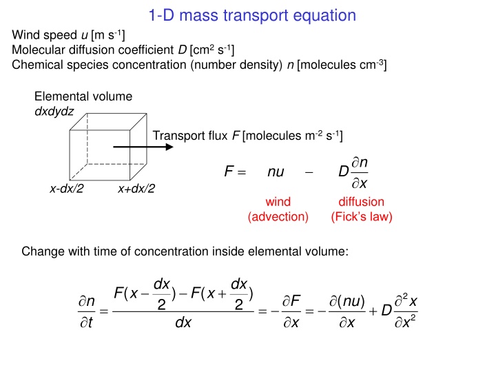
1-D mass transport equation Wind speed u [m s-1] Molecular diffusion coefficient D [cm2 s-1] Chemical species concentration (number density) n [molecules cm-3] Elemental volume dxdydz Transport flux F [molecules m-2 s-1] n x = F nu D x-dx/2 x+dx/2 wind diffusion (Fick s law) (advection) Change with time of concentration inside elemental volume: dx dx + F x ( ) F x ( ) 2 n t F x ( nu x ) x 2 2 = = = + D 2 dx x

Generalize mass transport equation to 3-D Fy Wind vector U = (u, v, w)T Flux vector F = (Fx, Fy, Fz)T Fz F = D n n F U Divergence operator Fx = )T ( / , / , / x y z Change of concentration with time: F y F x F z n t y = = = + D 2 ( n ) n F U x z x y 2 2 2 = + + 2 Laplacian 2 2 2 z

Advection vs. diffusion in driving atmospheric transport Time t needed for transport over distance L: Advection: t = L/U where U is wind speed Diffusion: t = L2/2D >>1: transport dominated by advection << 1: transport dominated by diffusion Peclet number: Pe = LU/D Typical values: L ~ 1 km U ~ 10 m s-1 D ~ 1/p ~ 0.1 cm2 s-1 at sea level Pe ~ 109 Diffusion is negligible

Different forms of the advection equation Eulerian flux form: n t = ( n ) U n is number density [molecules cm-3] Eulerian advective form: C t = C U C = n/nais mixing ratio [mol mol-1] where nais number density of air Compressibility of air ( 0) U affects number density, not mixing ratio Lagrangian form: dC dt d dt = 0 = + U where is the absolute derivative (for elemental volume moving with the flow) t Brasseur and Jacob, chap. 4.2.1

Adding source and sink terms: the continuity equation elemental volume transport chemistry Flux Fi = niU X Y Pi, Li deposition emission Continuity equations for number densities n = (n1, nK) of ensemble of K species: t local trend in number density (flux divergence) System of K coupled 4-D partial differential equations n Eulerian flux form + n ( ) i P ( ) L ) U n n i = ( i i emissions, deposition, chemical and aerosol processes transport Eulerian advective form: C t = U + C P L ( ) C ( ) C i i i i Lagrangian form dC dt = P L ( ) C ( ) C i i i Brasseur and Jacob, chap. 4.2.1

Break down dimensionality of continuity equation by operator splitting Solve for transport (x, y, z) and chemistry separately over finite time steps t C t = U + C P L ( ) C ( ) C i i i i Chemistry (local processes): Advection, further split in 1-D: = t C C x (Eulerian) u i i dC dt = P L ( ) C ( ) C i i i = (Lagrangian) Cy dx u t dt ( , ) x Cx C(t+ t) Cz C(t) t t t t Chemical equations: K-dimensional ODE system Advection equations: no chemical coupling Operator splitting induces error by ignoring couplings between transport in different directions and chemistry over t can quantify error by trying t /2, t/4, etc. Brasseur and Jacob, chap. 4.14

On-line and off-line approaches to chemical modeling On-line: coupled to dynamics Off-line: decoupled from dynamics GCM conservation equations: air mass: a / t = momentum: U/ t = heat: / t = water: q/ t = chemicals: Ci/ t = GCM conservation equations: air mass: a / t = momentum: U/ t = heat: / t = water: q/ t = meteorological archive (averaging time ~ hours) PROs of off-line vs on-line approach: computational cost simplicity stability (no chaos) compute sensitivities back in time CONs: no fast chemical-dynamics coupling need for meteorological archive transport errors Chemical transport model: Ci / t = Chemical data assimilation, forecasts best done on-line Chemical sensitivity studies may best be done off-line Brasseur and Jacob, chap. 1.7

Finite differencing in space: Eulerian models partition atmospheric domain into gridboxes This discretizes the continuity equation in space Solve continuity equation for individual gridboxes, like in a box model Present computational limit ~ 108 gridboxes In global models, this implies a grid resolution x of ~ 10-100 km in horizontal and 0.1-1 km in vertical Finite differencing in time and space are coupled by the Courant number condition = u t / x 1; in global models, t ~102-103 s The convenient orthogonal latitude-longitude grid suffers from Courant number singularity at poles Brasseur and Jacob, chap. 4.8

Eulerian models often use equal-area or zoomed grids Equal-area grids: avoid singularities at poles icosahedral triangular cubed-sphere Zoomed grids: increase resolution where you need it (or when, in an adaptive grid) nested stretched Brasseur and Jacob, chap. 4.8

Regional models: limited domain, boundary conditions at edges WRF domain with successive nests 2-way nesting 1-way nesting

Lagrangian models track points in model domain (no grid) Transport large number of points with trajectories from input meteorological data base (U) over time steps t Points have mixing ratio or mass but no volume Determine local concentrations in a given volume by the statistics of points within that volume or by interpolation PROS over Eulerian models: stable for any wind speed no error from spatial averaging easy to parallelize easily track air parcel histories efficient for receptor-oriented problems CONS: need very large # points for statistics inhomogeneous representation of domain individual trajectories do not mix cannot do nonlinear chemistry or aerosol physics cannot be conducted on-line with meteorology position to+ t U t position to Brasseur and Jacob, chap. 4.11

Lagrangian receptor-oriented modeling Run Lagrangian model backward from receptor location, with points released at receptor location only flow backward in time Efficient quantification of source influence distribution on receptor ( footprint )

Representing non-linear chemistry Consider two chemicals A and B emitted in different locations, and reacting by A + B products Eulerian model Lagrangian model gridboxes A B A B A and B never react A and B react following the mixing of gridboxes