Lauderdale County Virtual Academy 2023-2024 Orientation

Cost Economics
AAE 320
Paul D. Mitchell
Goal of Section
•
Overview what economists mean by Cost
•
(Economic) Cost Functions
–
Derivation of Cost Functions
–
Concept of Duality
–
What it all means
Economic Cost
•
Economic Cost: Value of what is given up
whenever an exchange or transformation of
resources takes place
•
For an exchange of resources (a purchase) not
only is money given up, but also the opportunity
to do some thing else with that money
•
For a transformation of resources (including
time), the opportunity to do other things with
those resources is given up
Economic Cost vs Accounting Cost
•
Economics includes these implicit costs in the
analysis that standard accounting methods do
not include
•
Accountants ask: What did you pay for it?
Explicit Cost
•
Economists
also
ask: What else could you do
with the money? Explicit Cost, plus Implicit
Cost (Opportunity Cost)
Economic Cost vs Accounting Cost
•
Economic cost ≠ accounting cost
•
Accounting Cost
: Used for financial reporting
(balancing the books, paying taxes, etc.)
–
Typically uses reported prices, wages and interest
rates (explicit costs)
•
Economic Costs
: Used for decision making
(resource allocation, developing strategy)
–
Includes opportunity costs (implicit costs) in the
analysis and calculates depreciation differently
Economic Cost vs Accounting Cost
•
Accounting Profit
= Revenue – Explicit Cost
•
Economic Profit
= Revenue – Explicit Cost
– Implicit Cost + Implicit Benefits
•
Economic analysis includes implicit costs and implicit
benefits that accounting does not include
•
Zero
economic
profit does not mean you are not
making money, but that you are making as much
money as you should, a “normal” rate of return
Opportunity Cost
•
Implicit Costs = “Opportunity Costs”
•
Value of the best opportunity given up because
resources are used for the given transaction or
transformation
•
“Value of the next best alternative”
•
Value of what you could do with your time & money
•
Opportunity Cost of Farming: Think of the Counter-
factual: What would you be doing if not farming?
•
Opportunity cost of your time
•
Opportunity cost of your assets and capital
Opportunity Cost
•
What’s your next best alternative?
•
Opportunity Cost of Time
Usually assume a different job and estimate
the implied lost wages
•
Opportunity Cost of Capital
Usually assume a low risk investment
alternative like bonds or CD and estimate
the implied lost returns on capital
•
Opportunity Cost of Asset (land)
Usually assume rental rate
Opportunity Cost of Time
•
Assume you make $50,000 as a farmer
•
Your next best job pays $45,000 = Opportunity Cost
of your Time as a farmer
•
Typical way of thinking: Accounting profit = $50,000
•
Economic way of thinking: look at difference in pay
•
Treat $45,000 as an “opportunity cost” and
subtract it from your current salary
Economic profit = $50,000 – $45,000 = $5,000
•
You are making $5,000 more with current job than
in your next best opportunity
Opportunity Cost of Capital
•
You have equity in your farm, your money invested in the farm
•
If you invest the money in a company (owned stock), bought
bonds, or a CD, they would pay you a dividend
•
We will use returns on these investments as a way to estimate
the opportunity cost of capital: you give up X% rate of return
•
What rate of return are you making by keeping your money in
the farm? Covered later in semester
•
Typical way of thinking: you have $100,000 equity in a farm,
earning 5% return = $5,000 annually
•
Economic way of thinking: treat the potential investment
income as an opportunity cost of capital: you could have
earned 3% in the bond market, so opportunity cost is $3,000
•
Economic profit = $5,000 – $3,000 = $2,000
Opportunity Cost of Working Assets
•
You have land and other “working assets” on a farm as well,
not just capital invested as equity
•
Instead of using them to farm, you could rent them out to
someone else at market rates, but still own them
–
Alternative opportunity to consider instead of the
conversion to “cash” in a hypothetical sale
•
This is the opportunity cost for you to use these assets to farm
•
Land, buildings, tractors, machinery, milk cows, breeding
livestock (bulls, cows, …)
•
You earn $300/acre growing crops, land rents for $200 in area
•
Accounting profit is $300/A, economic profit is $100/A
Economic Profit vs Accounting Profit
•
Accounting profit is the “normal” way of thinking: I make
$50,000 as a farmer, I earn a 5% rate of return on my farm
equity, I make $300/A growing crops
•
Economic profit: How do these compare to what else you
could make with these?
•
Alternatives: $45,000 salary, $100,000 at 3% = $3,000
investment, and $200/A land rent
•
You are making a positive economic profit: very good
•
$5000 more in salary, 2% more than market rates,
$100/acre more in return to land
•
If economic profit is zero, you are making as much as you
can—no better opportunities exist for you
Economic Benefits
•
Economic profit includes benefits accounting
methods do not
•
Accounting Profit = Revenue – Explicit Cost
•
Economic Profit
= Revenue – Explicit Cost – Implicit
Cost + Implicit Benefits
•
What benefits do you get from an activity besides
money?
•
Economics develops ways to estimate these types of
benefits or values based on available data
•
If you accept a below market salary/rate of return for
a job, you must be getting other economic benefits
Main point of this section
•
“Cost” in economics is more comprehensive
than accounting cost
•
Exposure to concept of opportunity cost
•
Start New Section: Cost Functions
Cost Definitions
•
Cost Function: schedule or equation that gives
the
minimum
cost to produce the given
output Q, e.g., C(Q)
•
Cost functions are not the sum of prices times
inputs used: C = r
x
X + r
y
Y
•
C = r
x
X + r
y
Y is cost as a function of the
inputs
X and Y, not cost as a function of
output
Q
Cost Functions
•
Output Price = Marginal Cost (P = MC)
identifies how much output Q to produce
•
Profit, production function and prices identify
inputs to use VMP = r, this gives output Q
•
Cost depends on inputs used and their prices,
but how much of each input to use?
•
Mathematical wonders of duality needed to
fully explain how it works
Main Point
•
If you choose Q so that price = marginal cost,
the inputs needed to produce this level of
output at minimum cost will satisfy the
optimality conditions we have already seen:
VMP
x
= r
x
and MP
x
/MP
y
= r
x
/r
y
•
Duality implies that a cost function with
standard properties implies a production
function with standard properties
Fixed Cost (FC)
•
Costs that do not vary with the level of output
Q during the planning period
•
Cost of resources committed through previous
planning
•
Property Taxes, Insurance, Depreciation,
Interest Payments, Scheduled Maintenance
•
In the long run, all costs are variable because
you can change assets
Variable Cost (VC)
•
Costs that change with the level of output Q
that is produced
•
Manager controls these costs
•
Fertilizer, Seed, Herbicides, Feed, Grain, Fuel,
Veterinary Services, Hired Labor
•
Vary the relative amounts used as increase
output produced
Cost Definitions
•
Total Cost TC = fixed cost + variable cost
•
Average Fixed Cost AFC = FC/Q
•
Average Variable Cost AVC = VC/Q
•
Average Total Cost ATC = TC/Q
•
Marginal Cost MC = cost of producing the last
unit of output = slope of the TC = slope of the
VC = dTC/dQ = dVC/dQ
Output Q
Cost
TC
FC
VC
Cost Function Graphics
Output Q
Cost
Average Costs = slope of line
through the origin to the point
on the function
TC
Output Q
Cost
VC
AVC
Minimum AVC
TC
ATC
Minimum ATC
Output Q
Cost
TC
VC
FC
MC
ATC
AVC
Cost Function Graphics
Output Q
Cost
MC
ATC
AVC
Cost Function Graphics
Livestock Example
•
Suppose you have pasture and will stock steers over
the summer to sell in the fall
•
As add more steers, eventually the rate of gain
decreases as forage per animal falls (diminishing
marginal product)
•
Fixed cost = $5,000 in land opportunity costs,
depreciation on fences and watering facilities,
insurance, property taxes, etc.
•
Variable cost = $495/steer: buying, transporting, vet
costs, feed supplements, etc.
Steers
Beef (cwt)
Marginal Product (cwt)
Production Function
Think Break #9 (Review)
How many steers should you
stock if the expected selling
price is $90/cwt and steers
cost $495 each?
Hint: What’s the single input
optimality condition?
Steers X
Costs $
Why aren’t these FC, VC and TC curves?
Beef Produced (cwt) Q
Costs $
TC
VC
FC
Because MP decreases, TC and VC increase more
and more rapidly as output increases (that’s duality)
Beef Produced (cwt) Q
Costs $
MC
ATC
AVC
Profit Maximization and
Cost Functions
•
Choose output Q to maximize profit
Max
= pQ – C(Q)
FOC: d
/dQ = p – MC(Q) = 0
Choose output Q so that price equals
marginal cost will maximize profit
SOC: d
2
/dQ
2
= – MC’(Q) < 0, or C’’(Q) > 0
Need a convex cost function (diminishing
marginal product)
P = MC and VMP = r
•
Cost Function based optimality condition
P = MC identifies Q = 475 cwt as the profit
maximizing output
•
To produce Q = 475 cwt requires 70 steers
•
Production Function based optimality
condition VMP = r identifies Steers = 70 as the
profit maximizing input use
•
Buying 70 steers produces Q = 475 cwt
•
Optimality conditions are consistent with each
other because of duality
marginal cost
increases because
marginal product
decreases
Think Break #10
•
You work for UWEX and have data on several farms
in your seven county district
•
You look at all farms with similar sized milking parlors
and a similar number of workers
•
You calculate the average production per cow as the
number of cows varies among the farms
•
Use these data in the table to recommend the
optimal milk output and herd size
Think Break #10
(VC = $3350/cow)
1)
Fill in the
missing MC’s
2)
If the milk
price is
$14/cwt, what
is the optimal
milk output
and farm size?
MC = Output Supply Curve
•
Maximize
= PQ – TC(Q) gives P = MC(Q)
•
P = MC(Q) defines the supply curve — for any price P,
how much output Q to supply
•
Profit changes along the MC curve, but for the given
price, the maximum is on the MC curve
•
Think of MC curve as a line defining the peak of a
long ridge, with the elevation of the peak (profit)
changing along the line
ATC defines Zero Profit
•
With free entry and exit and competition, long
run
economic
profit is zero—everyone earns a
fair return for their time & assets
•
Set profit to zero and rearrange
PQ – TC(Q) = 0 becomes PQ = TC(Q), then P =
TC(Q)/Q = ATC
•
P = ATC defines zero profit
•
Think of ATC curve as line defining sea level,
below ATC means
< 0
MC = ATC at min ATC
•
ATC = TC(Q)/Q, use quotient rule to get first
derivative, then set = 0 and solve
•
d(TC(Q)/Q)/dQ = (MC x Q – TC(Q))/Q
2
= 0
•
Rearrange to get MC x Q = TC(Q), and then MC =
TC(Q)/Q = ATC
•
FOC implies MC = ATC at min ATC
•
Intersection between MC and ATC occurs when
ATC is at a minimum
•
Min ATC: where profit max ridge hits the sea
MC = AVC at min AVC
•
Repeat process with AVC
•
d(VC(Q)/Q)/dQ = (MC x Q – VC(Q))/Q
2
= 0
•
Rearrange to get MC x Q = VC(Q), and then MC
= VC(Q)/Q = AVC
•
FOC implies MC = AVC at min AVC
•
Intersection between MC and AVC occurs when
AVC is at a minimum
Profit and min AVC
•
Profit at min AVC:
= PQ – VC(Q) – FC
•
P = MC = AVC at min AVC, so rewrite as
= MC x Q – VC(Q) – FC
•
VC(Q) = (VC(Q)/Q) x Q = AVC(Q) x Q, so
rewrite as
= MC x Q – AVC(Q) x Q – FC, or
=
Q(MC – AVC(Q)) – FC
•
MC = AVC at min AVC, so MC – AVC = 0, so
that
= – FC
•
Produce at P ≥ min AVC because, though lose
money, still pay part of FC
Cost Functions and Supply
MC
ATC
AVC
Green: P ≥ min ATC and
≥ 0
Yellow: min AVC ≤ P ≤ min ATC
and – FC ≤
≤ 0
Output Q
Cost or Price
Cost Function and Supply
Output Q
Cost or Price
MC
Green is complete supply schedule
AVC
ATC
Think Break #11
These are the
Think Break
#10 data (FC
= $10,000)
1)
Fill in the
missing costs
2)
What do you
recommend
for farms this
size if the
milk price is
$13/cwt?
What if P < min AVC?
•
Remember economic profit includes
opportunity costs, so negative economic profit
means better opportunities elsewhere
•
Your money/assets and time would get better
returns in other activities
•
Choices when p < min AVC for long term
1) Quit and convert resources
2) Find new way to produce with lower average
production costs (new technology)
Other Cost Terms Used
•
Fixed Cost synonyms: Overhead, Ownership Costs
•
Variable Costs synonyms : Operating Costs, Out-of-
Pocket Costs
•
Direct vs Indirect:
direct costs are linked to a specific
enterprise (dairy), indirect are not (pickup truck,
tractors). Both can be fixed and variable
•
Cash vs Non-Cash: Cash costs paid from farm income,
while non-cash costs include depreciation, returns to
equity, labor, management (opportunity costs). Both
can be fixed and variable
Summary
•
Opportunity Cost
•
Cost Functions
•
Definitions
•
Graphics
•
Profit Maximization and Cost Functions
•
Optimality conditions
•
Graphics
•
Output supply
Lauderdale County Virtual Academy 2023-2024 Orientation provides information about the academy, team members, lab schedule, student handbook, parent/guardian and student responsibilities. It includes details about the academy's location, team members, lab time schedule, and expectations for students and parents.

Download Presentation

Please find below an Image/Link to download the presentation.
The content on the website is provided AS IS for your information and personal use only. It may not be sold, licensed, or shared on other websites without obtaining consent from the author. Download presentation by click this link. If you encounter any issues during the download, it is possible that the publisher has removed the file from their server.
E N D
Presentation Transcript
Cost Economics AAE 320 Paul D. Mitchell
Goal of Section Overview what economists mean by Cost (Economic) Cost Functions Derivation of Cost Functions Concept of Duality What it all means
Economic Cost Economic Cost: Value of what is given up whenever an exchange or transformation of resources takes place For an exchange of resources (a purchase) not only is money given up, but also the opportunity to do some thing else with that money For a transformation of resources (including time), the opportunity to do other things with those resources is given up
Economic Cost vs Accounting Cost Economics includes these implicit costs in the analysis that standard accounting methods do not include Accountants ask: What did you pay for it? Explicit Cost Economists also ask: What else could you do with the money? Explicit Cost, plus Implicit Cost (Opportunity Cost)
Economic Cost vs Accounting Cost Economic cost accounting cost Accounting Cost: Used for financial reporting (balancing the books, paying taxes, etc.) Typically uses reported prices, wages and interest rates (explicit costs) Economic Costs: Used for decision making (resource allocation, developing strategy) Includes opportunity costs (implicit costs) in the analysis and calculates depreciation differently
Economic Cost vs Accounting Cost Accounting Profit = Revenue Explicit Cost Economic Profit = Revenue Explicit Cost Implicit Cost + Implicit Benefits Economic analysis includes implicit costs and implicit benefits that accounting does not include Zero economic profit does not mean you are not making money, but that you are making as much money as you should, a normal rate of return
Opportunity Cost Implicit Costs = Opportunity Costs Value of the best opportunity given up because resources are used for the given transaction or transformation Value of the next best alternative Value of what you could do with your time & money Opportunity Cost of Farming: Think of the Counter- factual: What would you be doing if not farming? Opportunity cost of your time Opportunity cost of your assets and capital
Opportunity Cost What s your next best alternative? Opportunity Cost of Time Usually assume a different job and estimate the implied lost wages Opportunity Cost of Capital Usually assume a low risk investment alternative like bonds or CD and estimate the implied lost returns on capital Opportunity Cost of Asset (land) Usually assume rental rate
Opportunity Cost of Time Assume you make $50,000 as a farmer Your next best job pays $45,000 = Opportunity Cost of your Time as a farmer Typical way of thinking: Accounting profit = $50,000 Economic way of thinking: look at difference in pay Treat $45,000 as an opportunity cost and subtract it from your current salary Economic profit = $50,000 $45,000 = $5,000 You are making $5,000 more with current job than in your next best opportunity
Opportunity Cost of Capital You have equity in your farm, your money invested in the farm If you invest the money in a company (owned stock), bought bonds, or a CD, they would pay you a dividend We will use returns on these investments as a way to estimate the opportunity cost of capital: you give up X% rate of return What rate of return are you making by keeping your money in the farm? Covered later in semester Typical way of thinking: you have $100,000 equity in a farm, earning 5% return = $5,000 annually Economic way of thinking: treat the potential investment income as an opportunity cost of capital: you could have earned 3% in the bond market, so opportunity cost is $3,000 Economic profit = $5,000 $3,000 = $2,000
Opportunity Cost of Working Assets You have land and other working assets on a farm as well, not just capital invested as equity Instead of using them to farm, you could rent them out to someone else at market rates, but still own them Alternative opportunity to consider instead of the conversion to cash in a hypothetical sale This is the opportunity cost for you to use these assets to farm Land, buildings, tractors, machinery, milk cows, breeding livestock (bulls, cows, ) You earn $300/acre growing crops, land rents for $200 in area Accounting profit is $300/A, economic profit is $100/A
Economic Profit vs Accounting Profit Accounting profit is the normal way of thinking: I make $50,000 as a farmer, I earn a 5% rate of return on my farm equity, I make $300/A growing crops Economic profit: How do these compare to what else you could make with these? Alternatives: $45,000 salary, $100,000 at 3% = $3,000 investment, and $200/A land rent You are making a positive economic profit: very good $5000 more in salary, 2% more than market rates, $100/acre more in return to land If economic profit is zero, you are making as much as you can no better opportunities exist for you
Economic Benefits Economic profit includes benefits accounting methods do not Accounting Profit = Revenue Explicit Cost Economic Profit = Revenue Explicit Cost Implicit Cost + Implicit Benefits What benefits do you get from an activity besides money? Economics develops ways to estimate these types of benefits or values based on available data If you accept a below market salary/rate of return for a job, you must be getting other economic benefits
Main point of this section Cost in economics is more comprehensive than accounting cost Exposure to concept of opportunity cost Start New Section: Cost Functions
Cost Definitions Cost Function: schedule or equation that gives the minimum cost to produce the given output Q, e.g., C(Q) Cost functions are not the sum of prices times inputs used: C = rxX + ryY C = rxX + ryY is cost as a function of the inputs X and Y, not cost as a function of output Q
Cost Functions Output Price = Marginal Cost (P = MC) identifies how much output Q to produce Profit, production function and prices identify inputs to use VMP = r, this gives output Q Cost depends on inputs used and their prices, but how much of each input to use? Mathematical wonders of duality needed to fully explain how it works
Main Point If you choose Q so that price = marginal cost, the inputs needed to produce this level of output at minimum cost will satisfy the optimality conditions we have already seen: VMPx= rxand MPx/MPy= rx/ry Duality implies that a cost function with standard properties implies a production function with standard properties
Fixed Cost (FC) Costs that do not vary with the level of output Q during the planning period Cost of resources committed through previous planning Property Taxes, Insurance, Depreciation, Interest Payments, Scheduled Maintenance In the long run, all costs are variable because you can change assets
Variable Cost (VC) Costs that change with the level of output Q that is produced Manager controls these costs Fertilizer, Seed, Herbicides, Feed, Grain, Fuel, Veterinary Services, Hired Labor Vary the relative amounts used as increase output produced
Cost Definitions Total Cost TC = fixed cost + variable cost Average Fixed Cost AFC = FC/Q Average Variable Cost AVC = VC/Q Average Total Cost ATC = TC/Q Marginal Cost MC = cost of producing the last unit of output = slope of the TC = slope of the VC = dTC/dQ = dVC/dQ
Cost Function Graphics TC VC Cost FC Output Q
TC Average Costs = slope of line through the origin to the point on the function Cost Output Q
TC VC Cost ATC AVC Minimum ATC Minimum AVC Output Q
Cost Function Graphics TC VC FC Cost 0 0 MC ATC AVC 0 Output Q 0
Cost Function Graphics MC Cost ATC AVC 0 Output Q 0
Livestock Example Suppose you have pasture and will stock steers over the summer to sell in the fall As add more steers, eventually the rate of gain decreases as forage per animal falls (diminishing marginal product) Fixed cost = $5,000 in land opportunity costs, depreciation on fences and watering facilities, insurance, property taxes, etc. Variable cost = $495/steer: buying, transporting, vet costs, feed supplements, etc.
Steers X Beef Q Production Function MP 700 0 0 600 Beef (cwt) 500 10 20 30 40 50 60 70 80 90 72 148 225 295 360 420 475 525 570 610 7.2 7.6 7.7 7.0 6.5 6.0 5.5 5.0 4.5 4.0 400 300 200 100 0 0 20 40 60 80 100 90 Marginal Product (cwt) 80 70 60 50 40 30 20 10 0 0 20 40 60 80 100 100 Steers
Think Break #9 (Review) Steers X Beef Q How many steers should you stock if the expected selling price is $90/cwt and steers cost $495 each? MP VMP 0 0 10 20 30 40 50 60 70 80 90 100 72 148 225 295 360 420 475 525 570 610 7.2 7.6 7.7 7.0 6.5 6.0 5.5 5.0 4.5 4.0 648 684 693 630 Hint: What s the single input optimality condition? 450 405 360
Steers X 0 10 20 30 40 50 60 70 80 90 100 Beef Q 0 72 148 225 295 360 420 475 525 570 610 F Cost V Cost Total C 5,000 5,000 4,950 5,000 9,900 14,900 66.89 100.68 5,000 14,850 19,850 66.00 5,000 19,800 24,800 67.12 5,000 24,750 29,750 68.75 5,000 29,700 34,700 70.71 5,000 34,650 39,650 72.95 5,000 39,600 44,600 75.43 5,000 44,550 49,550 78.16 5,000 49,500 54,500 81.15 AVC ATC MC 0 5,000 9,950 68.75 138.19 68.75 65.13 64.29 70.71 76.15 82.50 90.00 99.00 88.22 84.07 82.64 82.62 83.47 84.95 86.93 110.00 89.34 123.75
Why arent these FC, VC and TC curves? 60,000 50,000 40,000 Costs $ 30,000 20,000 10,000 0 0 20 40 60 80 100 Steers X
Because MP decreases, TC and VC increase more and more rapidly as output increases (that s duality) 60,000 TC 50,000 40,000 Costs $ VC 30,000 20,000 10,000 FC 0 0 100 200 Beef Produced (cwt) Q 300 400 500 600
140 ATC 120 MC 100 Costs $ 80 AVC 60 40 20 0 0 100 200 Beef Produced (cwt) Q 300 400 500 600
Profit Maximization and Cost Functions Choose output Q to maximize profit Max = pQ C(Q) FOC: d /dQ = p MC(Q) = 0 Choose output Q so that price equals marginal cost will maximize profit SOC: d2 /dQ2 = MC (Q) < 0, or C (Q) > 0 Need a convex cost function (diminishing marginal product)
Steers X Beef Q MP VMP F Cost V Cost Total C AVC ATC MC 0 0 5,000 0 5,000 10 72 7.2 648 5,000 4,950 9,950 68.75 138.19 68.75 20 148 7.6 684 5,000 9,900 14,900 66.89 100.68 65.13 30 225 7.7 693 5,000 14,850 19,850 66.00 88.22 64.29 40 295 7.0 630 5,000 19,800 24,800 67.12 84.07 70.71 50 360 6.5 585 5,000 24,750 29,750 68.75 82.64 76.15 60 420 6.0 540 5,000 29,700 34,700 70.71 82.62 82.50 70 475 5.5 495 5,000 34,650 39,650 72.95 83.47 90.00 80 525 5.0 450 5,000 39,600 44,600 75.43 84.95 99.00 90 570 4.5 405 5,000 44,550 49,550 78.16 86.93 110.00 100 610 4.0 360 5,000 49,500 54,500 81.15 89.34 123.75
P = MC and VMP = r Cost Function based optimality condition P = MC identifies Q = 475 cwt as the profit maximizing output To produce Q = 475 cwt requires 70 steers Production Function based optimality condition VMP = r identifies Steers = 70 as the profit maximizing input use Buying 70 steers produces Q = 475 cwt Optimality conditions are consistent with each other because of duality
90 80 Marginal Product (Beef cwt) 70 60 50 40 30 20 marginal cost increases because marginal product decreases 10 0 0 20 40 60 80 100 Input (Steers) 140 120 100 Marginal Cost 80 60 40 20 0 0 100 200 300 400 500 600 700 Output (Beef cwt)
Think Break #10 You work for UWEX and have data on several farms in your seven county district You look at all farms with similar sized milking parlors and a similar number of workers You calculate the average production per cow as the number of cows varies among the farms Use these data in the table to recommend the optimal milk output and herd size
Think Break #10 Cows Milk Q cwt (VC = $3350/cow) X 0 FC VC TC MC 0 10000 4800 10000 9640 10000 134000 144000 13.84 14490 10000 201000 211000 19320 10000 268000 278000 24100 10000 335000 345000 28824 10000 402000 412000 14.18 33488 10000 469000 479000 14.37 38096 10000 536000 546000 14.54 42624 10000 603000 613000 14.80 47060 10000 670000 680000 15.10 0 10000 77000 13.96 0 1) Fill in the missing MC s 20 40 60 80 100 120 140 160 180 200 67000 2) If the milk price is $14/cwt, what is the optimal milk output and farm size?
MC = Output Supply Curve Maximize = PQ TC(Q) gives P = MC(Q) P = MC(Q) defines the supply curve for any price P, how much output Q to supply Profit changes along the MC curve, but for the given price, the maximum is on the MC curve Think of MC curve as a line defining the peak of a long ridge, with the elevation of the peak (profit) changing along the line
ATC defines Zero Profit With free entry and exit and competition, long run economic profit is zero everyone earns a fair return for their time & assets Set profit to zero and rearrange PQ TC(Q) = 0 becomes PQ = TC(Q), then P = TC(Q)/Q = ATC P = ATC defines zero profit Think of ATC curve as line defining sea level, below ATC means < 0
MC = ATC at min ATC ATC = TC(Q)/Q, use quotient rule to get first derivative, then set = 0 and solve d(TC(Q)/Q)/dQ = (MC x Q TC(Q))/Q2 = 0 Rearrange to get MC x Q = TC(Q), and then MC = TC(Q)/Q = ATC FOC implies MC = ATC at min ATC Intersection between MC and ATC occurs when ATC is at a minimum Min ATC: where profit max ridge hits the sea
MC = AVC at min AVC Repeat process with AVC d(VC(Q)/Q)/dQ = (MC x Q VC(Q))/Q2 = 0 Rearrange to get MC x Q = VC(Q), and then MC = VC(Q)/Q = AVC FOC implies MC = AVC at min AVC Intersection between MC and AVC occurs when AVC is at a minimum
Profit and min AVC Profit at min AVC: = PQ VC(Q) FC P = MC = AVC at min AVC, so rewrite as = MC x Q VC(Q) FC VC(Q) = (VC(Q)/Q) x Q = AVC(Q) x Q, so rewrite as = MC x Q AVC(Q) x Q FC, or = Q(MC AVC(Q)) FC MC = AVC at min AVC, so MC AVC = 0, so that = FC Produce at P min AVC because, though lose money, still pay part of FC
Cost Functions and Supply Green: P min ATC and 0 MC Yellow: min AVC P min ATC and FC 0 Cost or Price ATC AVC 0 Output Q 0
Cost Function and Supply Green is complete supply schedule MC Cost or Price ATC AVC 0 Output Q 0
Think Break #11 These are the Think Break #10 data (FC = $10,000) Cows Milk VC TC MC ATC AVC 0 0 0 10000 77000 13.96 16.04 13.96 20 40 60 14490 201000 211000 13.81 14.56 80 19320 268000 278000 13.87 100 24100 335000 345000 14.02 120 28824 402000 412000 14.18 140 33488 469000 479000 14.37 14.30 14.01 160 38096 536000 546000 14.54 14.33 14.07 180 42624 603000 613000 14.80 14.38 14.15 200 47060 670000 680000 15.10 14.45 14.24 4800 9640 134000 144000 13.84 14.94 13.90 67000 1) Fill in the missing costs 2) What do you recommend for farms this size if the milk price is $13/cwt? 13.95
What if P < min AVC? Remember economic profit includes opportunity costs, so negative economic profit means better opportunities elsewhere Your money/assets and time would get better returns in other activities Choices when p < min AVC for long term 1) Quit and convert resources 2) Find new way to produce with lower average production costs (new technology)
Other Cost Terms Used Fixed Cost synonyms: Overhead, Ownership Costs Variable Costs synonyms : Operating Costs, Out-of- Pocket Costs Direct vs Indirect: direct costs are linked to a specific enterprise (dairy), indirect are not (pickup truck, tractors). Both can be fixed and variable Cash vs Non-Cash: Cash costs paid from farm income, while non-cash costs include depreciation, returns to equity, labor, management (opportunity costs). Both can be fixed and variable
Summary Opportunity Cost Cost Functions Definitions Graphics Profit Maximization and Cost Functions Optimality conditions Graphics Output supply


")
")


")