Kinematics in Physics: Equations, Graphs, and Definitions
Exploring kinematics in physics involves studying the motion of objects through equations, graphs, and definitions. Key concepts include position, distance, displacement, speed, velocity, and acceleration, along with scalar and vector quantities. Equations like s = (u + v)t and v = u + at are crucial for calculating motion parameters, while graphs like distance-time and velocity-time help in visualizing motion characteristics. This overview provides a comprehensive insight into the fundamentals of kinematics in physics.

Download Presentation

Please find below an Image/Link to download the presentation.
The content on the website is provided AS IS for your information and personal use only. It may not be sold, licensed, or shared on other websites without obtaining consent from the author.If you encounter any issues during the download, it is possible that the publisher has removed the file from their server.
You are allowed to download the files provided on this website for personal or commercial use, subject to the condition that they are used lawfully. All files are the property of their respective owners.
The content on the website is provided AS IS for your information and personal use only. It may not be sold, licensed, or shared on other websites without obtaining consent from the author.
E N D
Presentation Transcript
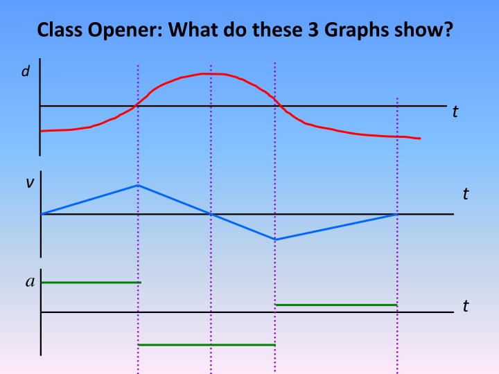
Class Opener: What do these 3 Graphs show? d t v t a t
Kinematic Equations Kinematics is the study of objects in Motion Grade 11 Physics NIS, Taldykorgan Mr. Marty
Objectives: Recall the definitions of position, distance, displacement, speed, velocity and acceleration and distinguish whether these are scalars or vectors. Use the equations of motion involving distance/displacement, speed/velocity, acceleration and time in calculations and in interpreting experimental results. Plot and interpret DTVA Graphs distance-time, velocity-time and acceleration-time graphs calculating the area under velocity-time graph to work out distance travelled for motion with constant velocity or constant acceleration.
Glossary- Kinematics English Definition Russian Kazakh Position The location of an object A scalar of the total amount of motion A vector that connects initial and final position of a moving body A scalar of how fast an object is moving A vector of rate of change of displacement Rate of change of velocity The rate of change of an incline Distance Displacement Speed Velocity Acceleration Gradient ,
Scalars and Vectors Scalar is a quantity that has only magnitude Vector is a quantity that has magnitude and direction Examples: distance time mass speed area work energy pressure Examples: displacement velocity acceleration force momentum electric field strength
Learners should know the equations: s = (u+v)t v = u +at v2= u2 +2as s = ut + at2 second, ms-2) t = time taken (seconds, s) Where: s = final displacement (metres) u = initial velocity (metres per second, ms-1) v = final velocity (ms-1) a = acceleration (metres per second per When 3 quantities are know the other 2 can be calculated These equations only apply during constant acceleration (motion is one-dimensional motion with uniform acceleration). When the acceleration is zero, s = ut.
Other symbols used in General Kinematic Equations Final velocity: vf = v0 + a(t) Distance traveled: d = v0 t + ( )at2 (Final velocity)2: vf2= (v0 t)2 + 2ad Distance traveled: d = [(v0 + vf)/2]*t
Calculus formulas Acceleration is the second derivative of displacement and velocity is the first derivative of displacement \dfrac{d^2s}{dt^2}=\dfrac{dv}{dt}=a Integration will give the area under a curve v=\dfrac{ds}{dt}=\int a\ dt = at + u
Slope of Distance-Time Graphs Motion is described by the equation d = vt The slope (gradient) of the DT graph = Velocity The steeper the line of a DT graph,the greater the velocity of the body 1 d(m) 2 3 v1 > v2 > v3 t(s)
Velocity-time Graphs Uniform accelerated motion is a motionwith the constant acceleration (a const) Slope (gradient) of the velocity time graph v(t) = acceleration The steeper the line of the graph v(t) the greater the acceleration of the body v(m/s) 1 2 3 t(s) a1 > a2 > a3
Graphing Negative Displacement B d 1 D Motion A t C A Starts at home (origin) and goes forward slowly B Not moving (position remains constant as time progresses) C Turns around and goes in the other direction quickly, passing up home
Tangent Lines show velocity d t On a position vs. time graph: SLOPE VELOCITY SLOPE SPEED Positive Positive Steep Fast Negative Negative Gentle Slow Zero Zero Flat Zero
Increasing & Decreasing Displacement d t Increasing Decreasing On a position vs. time graph: Increasing means moving forward (positive direction). Decreasing means moving backwards (negative direction).
d Concavity shows acceleration t On a position vs. time graph: Concave up means positive acceleration. Concave down means negative acceleration.
d Special Points Q R P t S Inflection Pt. Peak or Valley Time Axis Intercept P, R Q Change of concavity Turning point Times when you are at home P, S
Curve Summary d B C t A D Concave Up v > 0 a > 0 (A) Concave Down v > 0 a < 0 (B) Increasing v < 0 a > 0 (D) v < 0 a < 0 (C) Decreasing
All 3 Graphs d t v t a t
Graphing Tips d t v t Line up the graphs vertically. Draw vertical dashed lines at special points except intercepts. Map the slopes of the position graph onto the velocity graph. A red peak or valley means a blue time intercept.
Graphing Tips The same rules apply in making an acceleration graph from a velocity graph. Just graph the slopes! Note: a positive constant slope in blue means a positive constant green segment. The steeper the blue slope, the farther the green segment is from the time axis. v t a t
Real life Note how the v graph is pointy and the a graph skips. In real life, the blue points would be smooth curves and the green segments would be connected. In our class, however, we ll mainly deal with constant acceleration. v t a t
Area under a velocity graph forward area v t backward area Area above the time axis = forward (positive) displacement. Area below the time axis = backward (negative) displacement. Net area (above - below) = net displacement. Total area (above + below) = total distance traveled.
v forward area Area t backward area The areas above and below are about equal, so even though a significant distance may have been covered, the displacement is about zero, meaning the stopping point was near the starting point. The position graph shows this too. d t
References: http://www.thestudentroom.co.uk/wiki/Revisi on:Kinematics_- _Equations_of_Motion_for_Constant_Acceler ation https://www.csun.edu/science/credential/cse t/cset-physics/ppt/kinematics-graphing.ppt http://www.learnapphysics.com/index.html