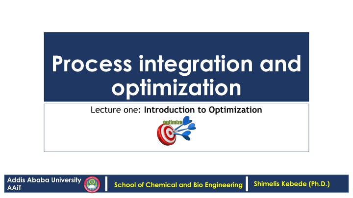
Introduction to Optimization in Process Engineering
Optimization in process engineering involves obtaining the best possible solution for a given process by minimizing or maximizing a specific performance criterion while considering various constraints. This process is crucial for achieving improved yields, reducing pollutants, energy consumption, and maintenance, and enhancing overall process understanding. The key ingredients of an optimization problem include decision variables, constraints, and the objective function. Constraints can be either equality or inequality constraints, depending on the specific requirements of the process. Understanding and applying optimization principles are essential for enhancing process efficiency and effectiveness in chemical and bioengineering.

Download Presentation

Please find below an Image/Link to download the presentation.
The content on the website is provided AS IS for your information and personal use only. It may not be sold, licensed, or shared on other websites without obtaining consent from the author.If you encounter any issues during the download, it is possible that the publisher has removed the file from their server.
You are allowed to download the files provided on this website for personal or commercial use, subject to the condition that they are used lawfully. All files are the property of their respective owners.
The content on the website is provided AS IS for your information and personal use only. It may not be sold, licensed, or shared on other websites without obtaining consent from the author.
E N D
Presentation Transcript
Process integration and optimization Lecture one: Introduction to Optimization Addis Ababa University AAiT Shimelis Kebede (Ph.D.) School of Chemical and Bio Engineering
OPTIMIZATION Optimization is a mathematical process of obtaining the minimum (or maximum) value of a function subject to some given constraints. Or A mathematical technique to find out the best possible solution You have a process that can be represented by a mathematical model. You also have a performance criterion such as minimum cost. The goal of optimisation is to find the values of the variables in the process that yield the best value of the performance criterion. Optimization involves searching for either the minimum or the maximum Addis Ababa University AAiT Shimelis Kebede (Ph.D.) School of Chemical and Bio Engineering
WHY OPTIMIZE? Improved yields, reduced pollutants Reduced energy consumption Higher processing rates Reduced maintenance, fewer shutdowns Better understanding of process (simulation) But there are always positive and negative factors to be weighed Addis Ababa University AAiT Shimelis Kebede (Ph.D.) School of Chemical and Bio Engineering
INGREDIENTS OF AN OPTIMISATION PROBLEM The following are the requirements for the application of optimization problems:- The design or decision variables the variables within a model that one can control The constraints (Performance criterion) The limit of any variable The objective function (cost function) the mathematical expression that we need to optimize Process model Process Mathematical presentation Addis Ababa University AAiT Shimelis Kebede (Ph.D.) School of Chemical and Bio Engineering
Performance criterion (constraints) Constraints are limitations on the values of decision variables. These may be linear or nonlinear, and they may involve more than one decision variable. When a constraint is written as an equality involving two or more decision variables, it is called an equality constraint. For example, a reaction may require a specific oxygen concentration in the combined feed to the reactor. The mole balance on the oxygen in the reactor feed is an equality constraint. Addis Ababa University AAiT Shimelis Kebede (Ph.D.) School of Chemical and Bio Engineering
Performance criterion (constraints) When a constraint is written as an inequality involving one or more decision variables, it is called an inequality constraint. For example, the catalyst may operate effectively only below 400 C, or below 20 MPa. Addis Ababa University AAiT Shimelis Kebede (Ph.D.) School of Chemical and Bio Engineering
Performance criterion (constraints) An equality constraint effectively reduces the dimensionality (the number of truly independent decision variables) of the optimization problem. Inequality constraints reduce (and often bound) the search space of the decision variables. Addis Ababa University AAiT Shimelis Kebede (Ph.D.) School of Chemical and Bio Engineering
Process or model (The objective function) (cost function) An objective function is a mathematical function that, for the best values of the decision variables, reaches a minimum (or a maximum). Thus, the objective function is the measure of value or goodness for the optimization problem. If it is a profit, one searches for its maximum. If it is a cost, one searches for its minimum. There may be more than one objective function for a given optimization problem. Addis Ababa University AAiT Shimelis Kebede (Ph.D.) School of Chemical and Bio Engineering
Some typical performance criteria: Maximum profit Minimum cost Minimum effort Minimum error Minimum waste Maximum throughput Best product quality Note the need to express the performance criterion in mathematical form. Addis Ababa University AAiT Shimelis Kebede (Ph.D.) School of Chemical and Bio Engineering
Optimisation Static optimisation: with respect to time. variables have numerical values, fixed Dynamic optimisation: variables are functions of time. Addis Ababa University AAiT Shimelis Kebede (Ph.D.) School of Chemical and Bio Engineering
Essential Features Every optimisation problem contains three essential categories: 1. 2. 3. At least one objective function to be optimised Equality constraints Inequality constraints Addis Ababa University AAiT Shimelis Kebede (Ph.D.) School of Chemical and Bio Engineering
Cont By a feasible solution we mean a set of variables which satisfy categories 2 and 3. The region of feasible solutions is called the feasible region. Addis Ababa University AAiT Shimelis Kebede (Ph.D.) School of Chemical and Bio Engineering
Cont An optimal solution is a set of values of the variables that are contained in the feasible region and also provide the best value of the objective function in category 1. For a meaningful optimisation problem the model needs to be underdetermined. Addis Ababa University AAiT Shimelis Kebede (Ph.D.) School of Chemical and Bio Engineering
Optimization and Chemical Engineering Optimization is important for process modelling, synthesis, design, operation and retrofitting of chemical, petrochemical, pharmaceutical, energy and related processes. Chemical engineers need to optimize the design and operating conditions of industrial process systems to improve their performance, costs, profitability, safety and reliability. Addis Ababa University AAiT Shimelis Kebede (Ph.D.) School of Chemical and Bio Engineering
Optimization and Chemical Engineering Process system optimization is challenging because chemical engineering application problems are often complex, nonlinear and large, have both equality and inequality constraints and/or involve both continuous and discrete decision variables. The mathematical relationships among the objective to be optimized and constraints and decision variables establish the difficulty and complexity of the optimization problem , as well as the optimization method that should be used for its solution. Addis Ababa University AAiT Shimelis Kebede (Ph.D.) School of Chemical and Bio Engineering
Optimization Applications Examples of optimization in a chemical plant: At what temperature to run a reactor? When to regenerate/change reactor catalyst? What distillation reflux ratio for desired purity? What pipe diameter for a piping network? Optimization can be used to determine the best answer to each of these questions Addis Ababa University AAiT Shimelis Kebede (Ph.D.) School of Chemical and Bio Engineering
Benefits of Optimization Able to systematically determine the best solution Model created for optimization can be used for other applications Insights gained during optimization process may identify changes that can be made to improve performance Addis Ababa University AAiT Shimelis Kebede (Ph.D.) School of Chemical and Bio Engineering
Optimization Requirements A clear understanding of what is needed to be optimized. Ex: minimize cost or maximize product quality? A clear understanding of the constraints on the optimization. Ex: safety concerns, customer requirements, budget limits, etc. A way to represent these mathematically (i.e. a model) Addis Ababa University AAiT Shimelis Kebede (Ph.D.) School of Chemical and Bio Engineering
More Definitions Minimum: A point where the objective function does not decrease when the variable(s) are changed some amount. Maximum: A point where the objective function does not increase when the variable(s) are changed some amount. Minimum Strict minimum: Addis Ababa University AAiT Shimelis Kebede (Ph.D.) School of Chemical and Bio Engineering
Minimization Vs Maximization Addis Ababa University AAiT Shimelis Kebede (Ph.D.) School of Chemical and Bio Engineering
Mathematical Description x Minimize : ( ) objective function ( ) Subject to: ( ) inequality constraints where , is a vector of n variables ( , , ( ) is a ve h x ctor of equalities of dimension ( ) is a vector of inequalities of dimension g x f = h x g x 0 0 equality constraints n x , ) x x x n 1 2 m 1 m 2 Addis Ababa University AAiT Shimelis Kebede (Ph.D.) School of Chemical and Bio Engineering
Steps Used To Solve Optimisation Problems 1.Analyse the process in order to make a list of all the variables. 2.Determine the optimisation criterion and specify the objective function. 3.Develop the mathematical model of the process to define the equality and inequality constraints. Identify the independent and dependent variables to obtain the number of degrees of freedom. Addis Ababa University AAiT Shimelis Kebede (Ph.D.) School of Chemical and Bio Engineering
Steps Used To Solve Optimisation Problems 1.If the problem formulation is too large or complex simplify it if possible. 2.Apply a suitable optimisation technique. 3.Check the result and examine it s sensitivity to changes in model parameters and assumptions. Addis Ababa University AAiT Shimelis Kebede (Ph.D.) School of Chemical and Bio Engineering
Modeling Example 1 A chemical plant makes urea and ammonium nitrate. The net profits are $1000 and $1500/ton produced respectively. Both chemicals are made in two steps reaction and drying. The number of hours necessary for each product is given below: Step/Chemical Urea Ammonium Nitrate Reaction 4 2 Drying 2 5 Addis Ababa University AAiT Shimelis Kebede (Ph.D.) School of Chemical and Bio Engineering
Cont The reaction step is available for a total of 80 hours per week and the drying step is available for 60 hours per week. There are 75 tons of raw material available. Each ton produced of either product requires 4 tons of raw material. What is the production rate of each chemical that will maximize the net profit of the plant? Addis Ababa University AAiT Shimelis Kebede (Ph.D.) School of Chemical and Bio Engineering
Cont Objective Function: We want to maximize the net profit. Net Profit = Revenue Cost. Let x1 = tons of urea produced per week & x2 = tons of ammonium nitrate produced per week. Revenue = 1000x1 + 1500x2. There is no data given for costs, so assume Cost = 0. So the objective function is: Maximize 1000x1 + 1500x2 Addis Ababa University AAiT Shimelis Kebede (Ph.D.) School of Chemical and Bio Engineering
Cont Constraints: We are given that the reaction step is available for 80 hrs/week. So, the combined reaction times required for each product cannot exceed this amount. The table says the each ton of urea produced requires 4 hours of reaction and each ton of ammonium nitrate produced requires 2 hours of reaction. This gives the constraint: 4x1 + 2x2 80 Addis Ababa University AAiT Shimelis Kebede (Ph.D.) School of Chemical and Bio Engineering
Cont We are also given that the drying step is available for 60 hrs/wk. The table says that urea requires 2 hrs/ton produced and ammonium nitrate requires 5 hrs/ton produced. So, we end up with the following constraint: 2x1 + 5x2 60 Addis Ababa University AAiT Shimelis Kebede (Ph.D.) School of Chemical and Bio Engineering
Cont We are given that the supply of raw material is 75 tons/week and each ton of urea or ammonium nitrate produced requires 4 tons of raw material. This gives our final constraint: 4x1 + 4x2 75 Addis Ababa University AAiT Shimelis Kebede (Ph.D.) School of Chemical and Bio Engineering
Cont Finally, to ensure a realistic result, it is always prudent to include non-negativity constraints for the variables where applicable. Here, we should not have negative production rates, so we include the two constraints x1 0 & x2 0 Addis Ababa University AAiT Shimelis Kebede (Ph.D.) School of Chemical and Bio Engineering
Cont So, we have the following problem: Maximize 1000x1 + 1500x2 Constraint 1 Constraint 2 Subject to: 4x1 + 2x2 80 When solved, this has an optimal answer of x1 = 11.25 tons/wk & x2 = 7.5 tons/wk 2x1 + 5x2 60 4x1 + 4x2 75 x1, x2 0 Constraint 3 Addis Ababa University AAiT Shimelis Kebede (Ph.D.) School of Chemical and Bio Engineering
Graph of Example 1 The grey area is called the feasible region and you can see that the optimum point is at the intersections of constraints 2 & 3. Since we are maximizing, we went in the direction of the profit vector Addis Ababa University AAiT Shimelis Kebede (Ph.D.) School of Chemical and Bio Engineering
Modeling Example 2 A company has three plants that produce ethanol and four customers they must deliver ethanol to. The following table gives the delivery costs per ton of ethanol from the plants to the customers. (A dash in the table indicates that a certain plant cannot deliver to a certain customer.) Plant/Customer C1 P1 132 P2 84 P3 106 C2 - C3 97 C4 103 91 - - 89 100 98 Addis Ababa University AAiT Shimelis Kebede (Ph.D.) School of Chemical and Bio Engineering
Cont.. The three plants P1, P2, & P3 produce 135, 56, and 93 tons/year, respectively. The four customers, C1, C2, C3, & C4 require 62, 83, 39, and 91 tons/year, respectively. Determine the transportation scheme that will result in the lowest cost. Addis Ababa University AAiT Shimelis Kebede (Ph.D.) School of Chemical and Bio Engineering
Cont.. Objective Function: We want to get the lowest cost, so we want to minimize the cost. The cost will be the costs given in the table times the amount transferred from each plant to each customer. Many of the amounts will be zero, but we must include them all because we don t know which ones we will use. Addis Ababa University AAiT Shimelis Kebede (Ph.D.) School of Chemical and Bio Engineering
Cont.. Let xij be the amount (tons/year) of ethanol transferred from plant Pi to customer Cj. So, x21 is the amount of ethanol sent from plant P2 to customer C1. We will leave out combinations the table says is impossible (like x12). So, the objective function is: Minimize 132 x11 + 97 x13 + 103 x14 + 84 x21 + 91 x22 + 106 x31 + 89 x32 + 100 x33 + 98 x34. Addis Ababa University AAiT Shimelis Kebede (Ph.D.) School of Chemical and Bio Engineering
Cont.. Constraints: The ethanol plants cannot produce more ethanol than their capacity limitations. The ethanol each plant produces is the sum of the ethanol it sends to the customers. So, for plant P1, the limit is 135 tons/year and the constraint is: x11 + x13 + x14 135 Since it can send ethanol to customers C1, C2, & C4. Addis Ababa University AAiT Shimelis Kebede (Ph.D.) School of Chemical and Bio Engineering
Cont.. For plants P2 & P3, the limits are 56 and 93 tons/year, so their constraints are: x21 + x22 56 x31 + x32 + x33 + x34 93 The sign is used because the plants may produce less than or even up to their limits, but they cannot produce more than the limit. Addis Ababa University AAiT Shimelis Kebede (Ph.D.) School of Chemical and Bio Engineering
Cont.. Also, each of the customers have ethanol requirements that must be met. For example, customer C1 must receive at least 62 tons/year from either plant P1, P2, P3, or a combination of the three. So, the customer constraint for C1 is: x11 + x21 + x31 62 Since it can receive ethanol from plants P1, P2, & P3. Addis Ababa University AAiT Shimelis Kebede (Ph.D.) School of Chemical and Bio Engineering
Cont.. The requirements for customers C2, C3, & C4 are 83, 39, & 91 tons/year so their constraints are: x22 + x32 83 x13 + x33 39 x14 + x34 91 The sign is used because it s alright if the customers receive extra ethanol, but they must receive at least their minimum requirements. Addis Ababa University AAiT Shimelis Kebede (Ph.D.) School of Chemical and Bio Engineering
Cont.. If the customers had to receive exactly their specified amount of ethanol, we would use equality constraints However, that is not stated for this problem, so we will leave them as inequality constraints Addis Ababa University AAiT Shimelis Kebede (Ph.D.) School of Chemical and Bio Engineering
Cont.. As in the last example, non-negativity constraints are needed because we cannot have a negative amount of ethanol transferred. x11, x13, x14, x21, x22, x31, x32, x33, x34 0 Addis Ababa University AAiT Shimelis Kebede (Ph.D.) School of Chemical and Bio Engineering
Cont.. The problem is: Minimize 132 x11 + 97 x13 + 103 x14 + 84 x21 + 91 x22 + 106 x31 + 89 x32 + 100 x33 + 98 x34 Subject to: x11+ x13 + x14 135 x21 + x22 56 x31 + x32 + x33 + x34 93 Addis Ababa University AAiT Shimelis Kebede (Ph.D.) School of Chemical and Bio Engineering
Cont.. x11 + x21 + x31 62 And: x11, x13, x14, x21, x22, x31, x32, x33, x34 0 x22 + x32 83 x13+ x33 39 x14 + x34 91 The optimum result is: x11 x13 x14 x21 x22 x31 x32 x33 x34 0 39 87 56 0 6 83 0 4 Addis Ababa University AAiT Shimelis Kebede (Ph.D.) School of Chemical and Bio Engineering
Cont.. Unlike the previous example, we cannot find the optimum point graphically because we have more than 2 variables This illustrates the power of mathematical optimization Addis Ababa University AAiT Shimelis Kebede (Ph.D.) School of Chemical and Bio Engineering
Classification of optimization techniques Classification based on presence/absence of constraint Constraint optimization problems: which are subjected to one or more constraint. Unconstraint optimization: in which no constraint exist Addis Ababa University AAiT Shimelis Kebede (Ph.D.) School of Chemical and Bio Engineering
Classification based on the nature of the equation involved: Linear programing (LP) Nonlinear programing (NLP) Quadratic programing (QP) Addis Ababa University AAiT Shimelis Kebede (Ph.D.) School of Chemical and Bio Engineering
Classification based on the nature of decision variables: Continuous optimization Integer programing (IP) Mixed integer linear programing (MILP) Mixed integer nonlinear programing (MINLP) Addis Ababa University AAiT Shimelis Kebede (Ph.D.) School of Chemical and Bio Engineering
Classification based on search space: Local search methods Global search methods Addis Ababa University AAiT Shimelis Kebede (Ph.D.) School of Chemical and Bio Engineering
Classification based on the number of objective function: Single objective optimization Multi-objective optimization Addis Ababa University AAiT Shimelis Kebede (Ph.D.) School of Chemical and Bio Engineering


")
")
")
 (cost")