Intense Muon Beams for Higgs Studies at ESS SB Project
The ESS SB project focuses on intense muon beams for studying the Higgs-related scalar sector. Key components include production, accumulation, cooling, and collider rings for Higgs studies. With a practical Higgs factory in mind, the facility features high-intensity H-source, p-compressor rings, ionization cooling system, LINAC acceleration, and colliders operating at L 10^32 cm^-2s^-1 and L 10^34 cm^-2s^-1. Proton intensity at ESS is crucial for the muon lifetime. GEANT4 simulations at 2.0 GeV involve charged pion and kaon production in a mercury target. The proton rings at ESS-LINAC can be doubled to 28 Hz. Accumilator and compressor rings manage 5 MWatt pulses with 1.5 ns proton pulses. To leverage ESS's power, secondary beam operation is subdivided into four pulses for efficient utilization. Tags: Intense Muon Beams, Higgs Studies, ESS SB Project, Collider Rings, GEANT4 Simulation

Download Presentation

Please find below an Image/Link to download the presentation.
The content on the website is provided AS IS for your information and personal use only. It may not be sold, licensed, or shared on other websites without obtaining consent from the author.If you encounter any issues during the download, it is possible that the publisher has removed the file from their server.
You are allowed to download the files provided on this website for personal or commercial use, subject to the condition that they are used lawfully. All files are the property of their respective owners.
The content on the website is provided AS IS for your information and personal use only. It may not be sold, licensed, or shared on other websites without obtaining consent from the author.
E N D
Presentation Transcript
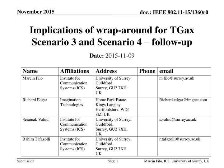
November 2015 doc.: IEEE 802.11-15/1360r0 Implications of wrap-around for TGax Scenario 3 and Scenario 4 follow-up Date: 2015-11-09 Name Marcin Filo Affiliations Address Institute for Communication Systems (ICS) Phone email University of Surrey, Guildford, Surrey, GU2 7XH. UK m.filo@surrey.ac.uk Richard Edgar Imagination Technologies Home Park Estate, Kings Langley, Hertfordshire, WD4 8lZ, UK University of Surrey, Guildford, Surrey, GU2 7XH. UK University of Surrey, Guildford, Surrey, GU2 7XH. UK Richard.edgar@imgtec.com Seiamak Vahid Institute for Communication Systems (ICS) Institute for Communication Systems (ICS) s.vahid@surrey.ac.uk Rahim Tafazolli r.tafazolli@surrey.ac.uk Submission Slide 1 Marcin Filo, ICS, University of Surrey, UK
November 2015 doc.: IEEE 802.11-15/1360r0 Abstract Implications of the use of Wrap-Around (WA) in TGax scenarios 3 and 4 are investigated. Simulations studies indicate significant differences in system performance with different number of simulated rings and also the need to reconsider some of the scenario specific simulation parameters. Direct follow up from IEEE 802.11-15/1049r1 [2]. Submission Slide 2 Marcin Filo, ICS, University of Surrey, UK
November 2015 doc.: IEEE 802.11-15/1360r0 SCE#3 and SCE#4 review SCE#3 (Indoor Small BSSs) and SCE#4 (Outdoor Large BSS Scenarios) represent planned real-world deployments which may consist of hundreds of BSSs To simplify simulation complexities hexagonal BSS layouts with a frequency reuse pattern are employed for both scenarios B S S B S S B S 10 11 9 B S S B S S B S S B S S 12 3 8 4 2 B S S ICD B S S B S S B S S B S S 13 19 1 5 7 B S S B S S B S S B S S 14 6 18 15 17 B S S B S S B S S 16 Figure 1. Layout of BSSs with Frequency reuse 1 Figure 2. Layout of BSSs using Frequency reuse 3 Submission Slide 3 Marcin Filo, ICS, University of Surrey, UK
November 2015 doc.: IEEE 802.11-15/1360r0 Problems with SCE#3 and SCE#4 hexagonal BSS layouts BSSs located in the outer ring behave differently from BSSs located in the inner rings. As a result, SCE#3 and SCE#4 hexagonal BSS layouts cannot be considered as a representative fraction of the actual deployments (i.e. we can assess performance only of the simulated layout, not the entire network) Additionally, SCE#3 and SCE#4 hexagonal BSS layouts assume only 2 rings which may not allow for proper evaluation of mechanisms for improving spatial reuse (e.g. a single AP transmission in SCE#3 may silence all other APs and STAs due to existence of a single collision domain) Submission Slide 4 Marcin Filo, ICS, University of Surrey, UK
November 2015 doc.: IEEE 802.11-15/1360r0 Possible solutions for problems with SCE#3 and SCE#4 hexagonal BSS layouts Solution 1: Simulate the entire deployment instead of just a fraction Requires definition of new BSS layouts with various number of rings and multiple simulation runs to cover a wide range of possible real-world deployments Solution 2: Simulate with wrap-around to minimize border effects With wrap-around no need to conduct multiple simulations for different BSS layout Submission Slide 5 Marcin Filo, ICS, University of Surrey, UK
November 2015 doc.: IEEE 802.11-15/1360r0 Wrap-around with simulations of CSMA based systems Issues related to the use of wrap-around, when used with insufficient number of rings: Over-estimation of spatial reuse happens when transmitters located outside of the boundaries of our network layout may trigger reception or CCA busy event in the central cell (specific for CSMA simulations) Over-estimation of network geometry happens when interferers located outside of the layout boundaries have a non-negligible impact on the SINR of the receivers located in the central cell (applicable to CSMA and non-CSMA simulations) Under-estimation of CSMA specific effect such as capture effect , hidden terminal problem , etc. Investigating the proper number of rings for simulations with wrap-around Main parameters affecting number of rings (scenario specific): Inter-cell distance (ICD), CCA-SD threshold/RX sensitivity, CCA-ED threshold, TX-power, Path-loss model Experimentally, simulations with different number of rings can help determine when the impact of the additional ring on the system performance can be neglected Submission Slide 6 Marcin Filo, ICS, University of Surrey, UK
November 2015 doc.: IEEE 802.11-15/1360r0 Wrap-around for SCE#3 and SCE#4 investigating proper number of rings Scenario 3 RX power seen by an AP in the second ring (from central AP) ~ -60dBm 217 BSSs 127 BSSs 169 BSSs 75% Other simulation settings: IEEE 802.11g (DSSS switched off), Shadowing and Fast fading not considered, No rate adaptation (Data/Control rate 24Mbps/24Mbps), CCA-SD threshold/RX sensitivity = -78dBm, CCA-ED threshold = -58dBm, STA density = 2000 STAs per km2, Full buffer (non-elastic traffic), Packet size = 1500B, Downlink only, Preamble reception model not considered Submission Slide 7 Marcin Filo, ICS, University of Surrey, UK
November 2015 doc.: IEEE 802.11-15/1360r0 Wrap-around for SCE#3 and SCE#4 investigating proper number of rings Scenario 4 127 BSSs 61 BSSs 91 BSSs 22.4% Other simulation settings: IEEE 802.11g (DSSS switched off), Shadowing and Fast fading not considered, Rate adaptation (Minstrel), CCA-SD threshold/RX sensitivity = -88dBm, CCA-ED threshold = -68dBm, STA density = 770 STAs per km2, Full buffer (non-elastic traffic), Packet size = 1500B, Downlink only, Preamble reception model not considered Submission Slide 8 Marcin Filo, ICS, University of Surrey, UK
November 2015 doc.: IEEE 802.11-15/1360r0 Wrap-around potential ways for reducing number of rings for SCE#3 and SCE#4 Scenario 3 Reduce power settings Increase Inter-Cell Distance (ICD) (e.g. simulations with reuse 3) 16% 61 BSSs 127 BSSs 91 BSSs 75% If we reduce power to 0dBm for APs and -5dBm for STA, difference between results for ring 2 and ring 11 drops to 16%, compared to75% for the original scenario settings Submission Slide 9 Marcin Filo, ICS, University of Surrey, UK
November 2015 doc.: IEEE 802.11-15/1360r0 Wrap-around potential ways for reducing number of rings for SCE#3 and SCE#4 Scenario 4 Introduce a PLOS cut-off to ensure that no two nodes can be in LOS after a certain distance (alternatively propose a new LOS probability function with a smaller tail) Increase ICD (simulations with reuse 3) Submission Slide 10 Marcin Filo, ICS, University of Surrey, UK
November 2015 doc.: IEEE 802.11-15/1360r0 Summary Wrap-around is necessary for proper evaluation of SCE#3 and SCE#4 (assuming we simulate just a small fraction of the actual deployment instead of the whole network) The accuracy of wrap-around technique depends to the size (i.e. number of rings) of the BSS layout Number of rings is scenario specific and may change depending on simulation settings (e.g. 11ax only deployment vs mixed deployment) Number of rings for SCE#3 and SCE#4 BSS layouts need to be sufficient to provide reliable results (if used with wrap-around) AP/STA power settings for SCE#3 may need to be reconsidered to reduce simulation complexity (if used with wrap-around) SCE#4 LOS probability function may need to be updated to reduce simulation complexity (if used with wrap-around) Submission Slide 11 Marcin Filo, ICS, University of Surrey, UK
November 2015 doc.: IEEE 802.11-15/1360r0 References [1] 11-14-0980-14-00ax, TGax Simulation Scenarios [2] IEEE 802.11-15/1049r1, Implications of wrap-around for TGax Scenario 3 and Scenario 3 (University of Surrey) Submission Slide 12 Marcin Filo, ICS, University of Surrey, UK
November 2015 doc.: IEEE 802.11-15/1360r0 Straw poll Should the table on Slide 13 be added to 11-14-980- 14-00ax (Section 3 and Section 4)? Y: N: A: Submission Slide 13 Marcin Filo, ICS, University of Surrey, UK
November 2015 doc.: IEEE 802.11-15/1360r0 Environment description BSSsare placed in a regular and symmetric grid as in Figure 6 for frequency reuse 1 and Figure 7 for frequency reuse 3. Each hexagon in Figures6 and 7 has the following configuration: Radius (R): 10 meters Inter BSS distance (ICD): 2*h meters h=sqrt(R2-R2/4) Wrap-around (radio-distance based) APs location AP Type Used with X number of rings (number of rings needs to be justified) / Not used AP is placed at the center of the hexagon,with 3m antenna height HEW Environment description Outdoor street deployment BSS layout configuration Define a 19 hexagonal grid as in Figure 9 With ICD = 130m h=sqrt(R2-R2/4)/2 Used with X number of rings (number of rings needs to be justified) / Not used Place APs on thecenter of each hexagon Antenna height 10m. HEW Wrap-around (radio-distance based) APs location AP Type Submission Slide 14 Marcin Filo, ICS, University of Surrey, UK
November 2015 doc.: IEEE 802.11-15/1360r0 Backup slides Submission Slide 15 Marcin Filo, ICS, University of Surrey, UK
November 2015 doc.: IEEE 802.11-15/1360r0 Wrap-around basics The original layout is extended to a cluster consisting of 6 displaced virtual copies of the original hexagonal network and the original hexagon network located in the center (see below) There is a one-to-one mapping between cells of the central (original) hexagonal network and cells of each copy (each copy have the same antenna configuration, traffic, power settings, etc.) Submission Slide 16 Marcin Filo, ICS, University of Surrey, UK
November 2015 doc.: IEEE 802.11-15/1360r0 Wrap-around basics Simple example: AP7 transmits a beacon frame and we want to determine the RX power of this beacon at AP13 1) Determine the RX power for the beacon as if it was transmitted from all 7 locations of AP7 2) Select the max RX power which in this case corresponds to AP7 location in C3 (assuming simple, distance dependent path-loss model with no shadowing and omni-directional antennas) Please note that for Radio distance based WA shortest distance does not always mean highest RX power! Submission Slide 17 Marcin Filo, ICS, University of Surrey, UK
November 2015 doc.: IEEE 802.11-15/1360r0 Main simulation parameter settings Main SCE#3 parameter settings as in [1] Inter-cell distance (ICD) = 17.32m (10m radius), AP/STA TX power = 20dBm / 15dBm Path-loss model as defined in [1] AP/STA antenna gain = 0.0dB / -2.0dB AP/STA noise figure = 7.0dB / 7.0 dB AP/STA antenna height = 3.0m / 1.5m Main SCE#4 parameter settings as in [1] Inter-cell distance (ICD) = 130 m (75m radius), AP/STA TX power = 20dBm / 15dBm Path-loss model as defined in [1] AP/STA antenna gain = 0.0dB / -2.0dB AP/STA noise figure = 7.0dB / 7.0 dB AP/STA antenna height = 10.0m / 1.5m Submission Slide 18 Marcin Filo, ICS, University of Surrey, UK
November 2015 doc.: IEEE 802.11-15/1360r0 Other simulation parameter settings Main simulation parameters Parameter Value Other IEEE 802.11 related parameters IEEE 802.11 standard IEEE 802.11g (DSSS switched off) Parameter Value Network layout Hexagonal grid Beacon period 100ms Wrap-around Yes (variable number of rings) STA/AP height As defined in [1] Probe timeout /Number of probe requests send per scanned channel 50ms / 2 STA distribution Random uniform distribution Modeling of preamble reception Not considered Scanning period (unassociated state only) Path loss model As defined in [1] 15s Shadow fading model Not considered RTS/CTS Off Fast fading model Not considered Packet fragmentation Off Mobility Not considered Number of orthogonal channels 1 The maximum number of retransmission attempts for a DATA packet Carrier frequency 2.4 GHz 7 Carrier bandwidth 20.0 MHz STA/AP Transmit power 15.0 dBm / 20.0 dBm Mistrel / -88.0 dBm (Scenario 4) -78.0 dBm (Scenario 3) Rate adaptation algorithm No Rate Adaptation (24Mbps/24Mbps) STA/AP Rx sensitivity STA/AP Noise Figure 7 dB MAC layer queue size 1000 packets STA/AP Antenna type Omni-directional STA/AP Antenna Gain -2.0 dBi / 0.0 dBi Number of beacons which must be consecutively missed by STA before disassociation 10 -68.0 dBm (Scenario 4) -58.0 dBm (Scenario 3) STA/AP CCA Mode1 threshold Strongest server (STAs always associate with APs with the strongest signal) STA-AP allocation rule Association Request Timeout / Number of Assoc Req. before entering scanning Traffic model Full buffer (saturated model) 0.5s / 3 Traffic type Non-elastic (UDP) Traffic direction Downlink only Transmission failure threshold for AP disassociation procedure Packet size (size of the packet transmitted on the air interface, i.e. with MAC, IP and TCP overheads) 0.99 1500 bytes (Application layer packet size: 1424 bytes) Submission Slide 19 Marcin Filo, ICS, University of Surrey, UK